Download
1 / 51
510 likes | 682 Views
ROMS data assimilation for ESPreSSO. Accomplishments:. * Nested ROMS in larger domain forward simulation (MABGOM-ROMS) with configuration suitable for IS4DVAR experimentation. Considerations: boundary conditions, resolution, computational cost

E N D
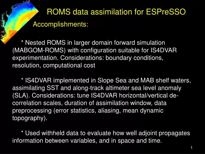
ROMS data assimilation for ESPreSSO Accomplishments: * Nested ROMS in larger domain forward simulation (MABGOM-ROMS) with configuration suitable for IS4DVAR experimentation. Considerations: boundary conditions, resolution, computational cost * IS4DVAR implemented in Slope Sea and MAB shelf waters, assimilating SST and along-track altimeter sea level anomaly (SLA). Considerations: tune IS4DVAR horizontal/vertical de-correlation scales, duration of assimilation window, data preprocessing (error statistics, aliasing, mean dynamic topography). * Used withheld data to evaluate how well adjoint propagates information between variables, and in space and time.
ROMS data assimilation for ESPreSSO Accomplishments: • * Full IS4DVAR reanalysis of NJ inner/mid-shelf for LaTTE using all data from CODAR, 2 gliders, moored current-meters and T/S, towed SeaSoar CTD, and satellite SST • * Developed adjoint-based analysis methods for observing system design and evaluation • * Have an ESPreSSO ROMS system ready for expansion to: • 2006-2008 reanalysis of ocean physics • introduction of in situ physical data into reanalysis • analyze impact of improved physics on ecosystem model • adjoint/tangent-linear simple optical model, with IS4DVAR
Mid-Atlantic Bight ROMS Model for ESPreSSO/IS4DVAR … ~12 km resolution outer model: NCOM global HyCOM/NCODA ROMS MAB-GoM 5 km resolution IS4DVAR model embedded in …
Mid-Atlantic Bight ROMS • 5 km resolution is for IS4DVARcan use 1 km downscale for forecast, with forward ecosystem/optics • 3-hour forecast meteorology NCEP/NAM • daily river flow (USGS) • boundary tides (TPX0.7) • nested in ROMS MABGOM V6 (nested in Global-HyCOM*) (* which assimilates altimetry) • nudging in a 30 km boundary zone • radiation of barotropic mode
Mid-Atlantic Bight ROMS Model for IS4DVAR 5 km resolution IS4DVAR model embedded in … … ROMS MAB-GoM V6 which uses global HyCOM+NCODA boundary data
Sequential assimilation of SLA and SST Before attempting assimilation of all in situ data for a full ESPreSSO reanalysis, we are assimilating satellite SSH and SST to tune for the assimilation parameters (horizontal and vertical de-correlation scales, duration of assimilation window, etc.) Unassimilated hydrographic data are used to evaluate how well the adjoint model propagates information between variables, and in space and time.
IS4DVAR* • Given a first guess (the forward trajectory)… • and given the available data… *Incremental Strong Constraint 4-Dimensional Variational data assimilation
IS4DVAR • Given a first guess (the forward trajectory)… • and given the available data… • what change (or increment) to the initial conditions (IC) produces a new forward trajectory that better fits the observations?
The best fit becomes the analysis assimilation window ti = analysis initial time tf = analysis final time The strong constraintrequires the trajectory satisfies the physics in ROMS. The Adjoint enforces the consistency among state variables.
The final analysis state becomes the IC for the forecast window assimilation window forecast tf = analysis final time tf + t = forecast horizon
Forecast verification is with respect to data not yet assimilated assimilation window forecast verification tf + t = forecast horizon
Basic IS4DVAR procedure: Lagrange function Lagrange multiplier J = model-data misfit The “best” simulation will minimize L: model model-data misfit is small and model physics are satisfied
Basic IS4DVAR procedure: Lagrange function Lagrange multiplier J = model-data misfit The “best” simulation minimizes L: At extrema of L we require:
Basic IS4DVAR procedure: (1) Choose an (2) Integrate NLROMS and save (a) Choose a (b) Integrate TLROMS and computeJ (c) Integrate ADROMS to yield (d) Compute (e) Use a descent algorithm to determine a “down gradient” correction to that will yield a smaller value of J (f) Back to (b) until converged (3) Compute new and back to (2) until converged J = model-data misfit Outer-loop (10) Inner-loop (3) NLROMS = Non-linear forward model; TLROMS = Tangent linear; ADROMS = Adjoint
xb= model state (background) at end of previous cycle, and 1st guess for the next forecast In 4D-Var assimilation the adjoint gives the sensitivity of the initial conditions to mis-match between model and data A descent algorithm uses this sensitivity to iteratively update the initial conditions, xa, (analysis) to minimize Jb+ S(Jo) xb previous forecast 0 1 2 3 4 time Observations minus Previous Forecast Adjoint model integration is forced by the model-data error dx
Observed information (e.g. SLA, SST) is transferred tounobserved state variables andprojected from surface to subsurface in 3 ways: (1) The Adjoint Model (2) Empirical statistical correlations to generate “synthetic XBT/CTD” • In EAC assimilation get T(z),S(z) from vertical EOFs of historical CTD observations regressed on SSH and SST (3) Modeling of the background covariance matrix • e.g. via the hydrostatic/geostrophic relation
MAB Satellite Observations for IS4DVAR • SST 5-km daily blended MW+IR from NOAA PFEG Coastwatch • MAB Sea Level Anomaly (SLA) is strongly anisotropic with short length scales due to flow-topography interaction, so use along-track altimetry (need coastal altimetry corrections for shelf data) • 4DVar uses all data at time of satellite pass • model “grids” data by simultaneously matching observations and dynamical and kinematic constraints 5 km resolution for IS4DVAR1 km downscale for forecast
Mid-Atlantic Bight ROMS Model for IS4DVAR Model variance (without assimilation) is comparable to along-track in Slope Sea, but not shelf-break AVISO gridded SLA differs from along-track SLA in Slope Sea (4 cm) and Gulf Stream (10 cm)
All inputs: NAM Ocean model based open boundary conditions River discharge, temperature (USGS) Altimetry (via RADS; AVISO gridded) XBT, CTD, Argo Satellite SST – IR and mWave, passes/blended HF radar – totals/radials Cabled observatory time series – MVCO Glider CTD (and optics) NDBC buoy time series (T, S, velocity) tide gauges waves Drifters - SLDMB and AOML GDP Delayed mode Oleander ADCP science moorings
Assimilation of hydrographic climatology for: * mean dynamic topography (altimetry) * removing model bias • Bias in the background state adversely affects how IS4DVAR projects model-data misfit across variables and dimensions • We assimilate a high-resolution (~2-5 km) regional temp/salt climatology to (i) produce a Mean Dynamic Topography (SSH) consistent with model physics, and (ii) to remove bias • Climatology computed by weighted least squares (Dunn et al. 2002, JAOT) from all available T-S data (NODC, NMFS) prior to 2006 (Naomi Fleming) • Three simulations: • ROMS nested in MABGOM V6 • Free running ROMS initialized with climatology and forced by climatology at the boundaries and mean surface wind stress • ROMS with climatology initial/boundary/forcing and assimilation of climatology over a 2-day window
Skill of climatologies and MABGOM-V6 at reproducing all XBT/CTD from GTS in 2007-2008 in Slope Sea
Skill of climatologies and MABGOM-V6 at reproducing all XBT/CTD from GTS in 2007-2008 in MAB shelf waters
Mean barotropic velocity from ROMS versus mean alongshelf velocity from analysis of mooring observations by Lentz (2008) Blue – mean of ROMS v6 Red – mean of clim ROMS Black – mean of assim ROMS Green - observations
High frequency variability: model and data issues ROMS includes high frequency variability typically removed in altimeter processing (tides, storm surge) The IS4DVAR cost function, J, samples this high frequency variability, so it must be either (a) removed from the model or (b) included in the data • Our approach: • Run 1-year ROMS (no assimilation) forced by boundary TPX0.7 tides; compute ROMS tidal harmonics • de-tide along-track altimetry (developmental in MAB) • add ROMS tides to de-tided altimeter data • thus the observations are adjusted to include model tide • assimilate – high frequency mismatch of model and altimeter is minimized and cost function is, presumably, dominated by sub-inertial frequency dynamics
High frequency variability: model and data issues The IS4DVAR increment is to the initial conditions of the analysis window, and this itself generates HF variability (inertial oscillations)
High frequency variability: model and data issues The IS4DVAR increment is to the initial conditions of the analysis window, and this itself generates HF variability (inertial oscillations) • Our approach: • Apply a short time-domain filter to IS4DVAR initial conditions • Reduces inertial oscillations in the Slope Sea but removes tides • Tides recover quickly • – approach needs refinement – possibly using 3-D velocity harmonic analysis of free running model
High frequency variability: model and data issues Without a subsurface synthetic-CTD relationship, the adjoint model can erroneously accommodate too much of the SLA model-data misfit in the barotropic mode This sends gravity wave at along the model perimeter • Our approach: • Repeat (duplicate) the altimeter SLA observations at t = -6 hour, t=0 and t = +6 hour but with appropriate time lags in the added tide signal • These data cannot easily be matched by a wave • We are effectively acknowledging the temporal correlation of the sub-tidal altimeter SLA data
High frequency variability: model and data issues • Our approach: • Repeat (duplicate) the altimeter SLA observations at t = -6 hour, t=0 and t = +6 hour but with appropriate time lags in the added tide signal • These data cannot easily be matched by a wave • We are effectively acknowledging the temporal correlation of the sub-tidal altimeter SLA data
Sequential assimilation of SLA and SST Before attempting assimilation of all in situ data for a full ESPreSSO reanalysis, we are assimilating satellite SSH and SST to tune for the assimilation parameters (horizontal and vertical de-correlation scales, duration of assimilation window, etc.) Unassimilated hydrographic data are used to evaluate how well the adjoint model propagates information between variables, and in space and time.
Sequential assimilation of SLA and SST • Reference time is days after 01-01-2006 • 3-day assimilation • window (AW) • Daily MW+IR blended SST (available real time) • SSH = Dynamic topography + ROMS tides + Jason-1 SLA (repeated three times) • For the first AW we just assimilate SST to allow the tides to ramp up.
Sequential assimilation of SLA and SST Assimilation window (3<=t<=6 days) ROMS SST and currents at 200 m ObservedSST XBT transect (NOT assimilated) Jason-1 data
Sequential assimilation of SLA and SST ROMS solutions along the transect positions [lon,lat,time]
Sequential assimilation of SLA and SST ROMS-IS4DVAR fits the surface observations (SST and SSH), but how well does it represent unassimilated subsurface data? ROMS solutions along the transect positions [lon,lat,time]
Forward model Assimilation of SST and SSH (no climatology bias correction) depth (m) depth (m)
ROMS data assimilation for ESPreSSO Accomplishments: • * Have a system ready for: • introduction of in situ physical data into reanalysis • 2006-2008 reanalysis of ocean physics • analysis of impact of improved physics on ecosystem (‘fasham’) and optical models • construction of adjoint/tangent-linear of optical model, and subsequent addition of optical data to cost function and full IS4DVAR
IS4DVAR data assimilation LaTTE: The Lagrangian Transport and Transformation Experiment system set-up: • resolution: 2.5km • forcing: NAM model output • rivers: USGS Hudson & Delaware gauges • DA window: 3 days • period: Apr. 10 – Jun 6, 2006 algorithm: Incremental Strong-constraint 4DVAR (Courtier et al, 1994, QJRMS; Weaver et al, 2003, MWR; Powell et al, 2008, Ocean Modelling) types and numbers of obs.
IS4DVAR result---- reduction of misfit 2006-04-20 06:57:36 evolution of cost function model observation
Ensemble measure of the influence of glider MURI track at the end of the glider mission Cost function: Covariance between J and temperature, , reflects the influence of glider observation, as plotted in the right. t: the finish time of a glider mission.
Ensemble measure of the influence of glider MURI track 5 days after the glider mission t: 5 days after the mission is finished.
Observation evaluation Assuming: model error ~ ocean state anomaly