Download
1 / 37
370 likes | 381 Views
COSTS OF PRODUCTION. General principle: If you know the technology of production (the production function or total product curve), and if you know the prices of the inputs to production, then you can find the firm’s costs at any level of output. Put another way:.

E N D
COSTS OF PRODUCTION • General principle: If you know the technology of production (the production function or total product curve), and if you know the prices of the inputs to production, then you can find the firm’s costs at any level of output. Short-run costs
Put another way: • Costs are determined by the technology of production and input prices. Let’s start with the total product curve for tax preparation services from the last section, and show how to get to costs of production. Short-run costs
Suppose labor costs $48 per day. • PL = $48/day • If labor is the only variable input, we can find the total variable costs at each output level. Short-run costs
TOTAL P L = L LABOR PRODUCT TVC 0 0 0 1 3 48 2 15 96 3 36 144 4 48 192 5 56 6 62 7 66 8 68 384 Short-run costs
THE TOTAL VARIABLE COST CURVE shows the total variable cost at each level of output. • In the total variable cost curve the independent variable is OUTPUT, and the dependent variable is TOTAL VARIABLE COSTS. Short-run costs
PLOT THE REST OF THE POINTS TO SHOW TVC. $ 700 When output is 56, total variable costs are $240. 600 500 400 300 200 100 0 Q 0 20 40 60 80 Short-run costs
If there are fixed costs (costs associated with inputs that can’t be changed), then we can add these to the total variable costs to get total costs. • Total Cost = Fixed Cost + Total Variable Cost • TC = FC + TVC Short-run costs
The total cost curve shows the total cost of producing each output. $ 700 600 TC 500 TVC 400 300 200 100 Q 0 20 40 60 80 Short-run costs
Here’s another total cost curve that we’ll use to introduce the concepts of average cost and marginal cost. Short-run costs
TC($) TC 700 600 500 400 300 200 100 0 0 2 4 6 8 10 12 14 Short-run costs
AVERAGE COST • Average cost: Cost per unit of output. Total cost divided by output. TC/Q. • Average cost curve: The curve that shows average cost as a function of output. Output is the independent variable and average cost is the dependent variable. Short-run costs
Q TC AC 0 50.0 AC = TC/Q = 97/5 1 63.0 63.0 2 71.0 35.5 3 76.0 25.3 4 82.4 20.6 5 97.0 19.4 6 130.0 7 174.0 8 233.0 9 314.0 34.9 10 460.0 46.0 11 656.0 59.6 Short-run costs
PLOT THE REST OF THE AC CURVE. AC($/Q) 120 100 80 AC 60 40 20 0 Q 0 2 4 6 8 10 12 14 Short-run costs
AVERAGE VARIABLE COSTS CAN BE SHOWN AT THE SAME TIME. Short-run costs
$/Q 120 100 80 AC 60 AVC 40 20 Q 0 0 2 4 6 8 10 12 14 Short-run costs
MARGINAL COST • Marginal cost: The change in total cost per unit change in output. The increase in cost due to producing one more unit of output. The slope of the total cost curve. TC / Q. • Marginal cost curve: The curve that shows marginal cost as a function of output. The independent variable is output. The dependent variable is marginal cost. Short-run costs
Q TC AC MC 0 50.0 1 63.0 63.0 13 2 71.0 35.5 8 The marginal cost of the 4th unit of output is 6.4 =(82.4-76)/(4-3) 3 76.0 25.3 5 4 82.4 20.6 6.4 5 97.0 19.4 14.6 6 130.0 21.7 33 7 174.0 24.9 8 233.0 29.1 9 314.0 34.9 10 460.0 46.0 146 11 656.0 59.6 196 Short-run costs
AC, MC MC 120 100 AC 80 AC 60 40 Q 20 0 0 2 4 6 8 10 12 14 Short-run costs
Of course, the marginal and average cost curves must conform to the usual rules about marginal and average curves. • 1) When the average is rising, the marginal quantity must be greater than the average quantity. • 2) When the average is falling, the marginal quantity must be less than the average quantity. • 3) When the average is neither rising nor falling (at a maximum or minimum), average and marginal are equal. Short-run costs
Notice that the general shape of the AC and MC curves can be deduced by looking as the TC curve. • (Review, if necessary, the techniques for finding AP and MP curves by inspecting TP curves covered in the last section.) Short-run costs
WHAT WOULD THE AVERAGE VARIABLE COST CURVE LOOK LIKE IF WE WERE TO PUT IT ON THE SAME DIAGRAM? $/Q MC 120 100 80 AC 60 40 20 0 Q 0 2 4 6 8 10 12 14 Short-run costs
$ TC 700 600 500 400 300 200 100 Q 0 Two alternative ways of showing information about the firm’s costs. 0 2 4 6 8 10 12 14 $/Q MC 120 100 80 AC 60 40 20 Q 0 0 2 4 6 8 10 12 14 Short-run costs
COST CURVE SUMMARY: • Costs depend output, technology, and input prices. • There are two ways to depict a firm’s costs: • 1) Total cost curves • 2) Average and marginal cost curves Short-run costs
CHANGES IN COSTS • What are the effects on costs of changes in • a) input prices? • b) the technology of production? • c) taxes on output? Short-run costs
What are the effects on a firm’s costs of an increase in the price of an input? • The increase in the price of a variable input will raise the total variable costs of production at each output level. • This has the effect of raising both marginal and average costs. Short-run costs
$ TC’ is the total cost curve when the price of a variable input is increased. TC’ 350 300 TC 250 200 150 100 50 0 Q 0 2 4 6 8 10 12 14 Increasing the price of an input raises both average and marginal costs. $/Q 60 MC’ 50 MC 40 AC’ 30 AC’ and MC’ show the effect of higher input prices. AC 20 10 0 Q 0 2 4 6 8 10 12 14 Short-run costs
An improvement in technology lowers the cost of producing each level of output. • Marginal and average costs of production will be lower as a result. Short-run costs
$ TC 350 300 IMPROVEMENTS IN TECHNOLOGY REDUCE COSTS OF PRODUCTION. TC’ 250 200 150 100 50 Q 0 Costs fall because the same output can be produced using fewer inputs. 0 2 4 6 8 10 12 14 $/Q 60 MC 50 MC’ 40 AC 30 AC’ 20 10 0 Q 0 2 4 6 8 10 12 14 Short-run costs
Imposing a tax per unit of output will raise total cost by tQ, where t is the tax per unit and Q is the number of units of output sold. • The tax will raise both average and marginal costs by exactly the amount of the tax per unit of output. Short-run costs
$ TC+3Q 350 300 TC A per unit tax of $3 will raise total cost by $3Q, or $3 times the quantity produced. 250 200 150 100 50 0 Q 0 2 4 6 8 10 12 14 $/Q 60 MC+3 A per unit tax of $3 will raise average and marginal cost by exactly $3. 50 MC 40 AC+3 30 AC 20 10 Q 0 0 2 4 6 8 10 12 14 Short-run costs
What is a SUBSIDY, and how does a per unit subsidy affect a firm’s costs? Short-run costs
$ • CHECK UP: WHAT DO THE AC AND MC CURVES LOOK LIKE FOR THE FOLLOWING TOTAL COST CURVES? TC Q Short-run costs
$ TC Q Short-run costs
$ TC Q Short-run costs
SUMMARY • Increases in the prices of inputs will raise the total, average, and marginal costs of production. • Improvements in technology lower total, average, and marginal costs of production. • A per unit tax of t will raise total costs by tQ, and will raise marginal and average costs by exactly t. Short-run costs