Download
1 / 32
320 likes | 426 Views
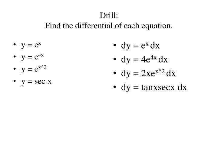
Drill: Find the differential of each equation. y = e x y = e 4x y = e x^2 y = sec x. dy = e x dx dy = 4e 4x dx dy = 2xe x^2 dx dy = tanxsecx dx. Slope Fields and Euler’s Method. Lesson 6.1. Objectives. Students will be able to:

E N D
Drill: Find the differential of each equation. • y = ex • y = e4x • y = ex^2 • y = sec x • dy = ex dx • dy = 4e4x dx • dy = 2xex^2 dx • dy = tanxsecxdx
Slope Fields and Euler’s Method Lesson 6.1
Objectives • Students will be able to: • construct antiderivatives using the Fundamental Theorem of Calculus. • solve initial value problems in the form • construct slope fields using technology and interpret slope fields as visualizations of different equations. • use Euler’s Method for graphing a solution to an initial value problem.
Differential Equation • An equation involving a derivative is called a differential equation. The order of a differential equation is the order of the highest derivative involved in the equation.
Example Solving a Differential Equation • Find all functions y that satisfy • Solution: the anti-derivative of dy/dx: • This is called a GENERAL solution. • We cannot find a UNIQUE solution unless we are given further information.
If the general solution to the first order differential equation is continuous, the only information needed is the value of the function at a single point, called an INITIAL CONDITION. • A differential equation with an initial condition is called an INITIAL VALUE PROBLEM. • It has a unique solution, called the PARTICULAR SOLUTION to the differential equation.
Example Solving a Differential Equation Find all the functions y that satisfy
Example Solving an Initial Value Problem Find the particular solution to the equation whose graph passes through the point (0, 1).
Example Solving an Initial Value Problem Find the particular solution to the equation and y = 60 when x = 4.
Example Handling Discontinuity • Find the particular solution to the equation dy/dx = 2x – sec2x whose graph passes through the point (0, 3) • The general solution is y = x2 – tanx + C • Applying the initial condition: 3 = 02 – tan0 + C; 3 = C • Therefore, the particular solution is y = x2 – tanx + 3 • However, since because tanx is does have discontinuities, you need to add the domain stipulation of –π/2 < x< π/2
Example Using the Fundamental Theorem • Find the solution to the differential equation f’(x) = e-x^2 for which f(7) = 3 • Rather than determining the anti-derivative, you can let the solution in integral form: • We know that if • Then AND • f’(x) = e-x^2 This is our solution! Note: If you are ABLE to determine the anti-derivative, you should do so!
Drill: Find the constant C • y = 3x2 + 4x + C and y = 2 when x = 1 • y = 2sinx – 3cosx + C and y = 4 when x = 0 • 2 = 3(1)2 + 4(1) + C • 2=3+4+C • 2 = 7 + C • -5 = C • 4 = 2sin(0) – 3cos(0) + C • 4 = 0 – 3 + C • 4 = -3 + C • 7 = C
Graphing a General Solution Note: you can also use the calc by putting values of ‘C’ in to L1 and then graphing y1 = sinx + L1 • Graph the family of functions that solve the differential equation dy/dx = cos x • Any function of the form y = sinx + C solves the differential equation. • First graph y = sin x, and then repeat the graph by shifting vertically up and down.
Slope Fields • a slope field (or direction field) is a graphical representation of the solutions of a first-order differential equation. It is achieved without solving the differential equation analytically. The representation may be used to qualitatively visualize solutions, or to numerically approximate them. • Remember also, that the derivative of a function gives its slope. • Also remember that we use the notation dy/dx to represent derivative; therefore, dy/dx = slope.
A Summary of Making Slope Fields • Put the differential equation in the form dy/dx = g(x,y) • Decide upon what rectangular region of the plane you want to make the picture • Impose a grid on this region • Calculate the value of the slope, g(x,y), at each grid point, (x,y) • Sketch a picture in which at each grid point there is a short line segment having the corresponding slope
Example: Constructing a Slope Field • Construct a slope field for the differential equation dy/dx = cos x • We know that that slope at any point (0, y) will be cos (0) = 1, so we can start be drawing tiny segments with slope 1 at several points along the y-axis. • Slope is also 1 at 2π, -2π • When would the slope by -1? • At π, - π • When is the slope 0? • At π/2, - π/2 • At 3π/2, -3π/2
Example Matching Slope Fields with Differential Equations Use slope analysis to match the differential equation with the given slope fields. Note: each block is .5 units.
Example Matching Slope Fields with Differential Equations Use slope analysis to match the differential equation with the given slope fields. Note: each block is .5 units
Example Matching Slope Fields with Differential Equations Use slope analysis to match the differential equation with the given slope fields. Note: each block is .5 units
Example Matching Slope Fields with Differential Equations Use slope analysis to match the differential equation with the given slope fields. Note: each block is .5 units
Example Matching Slope Fields with Differential Equations Use slope analysis to match the differential equation with the given slope fields. Note: each block is .5 units
Example Matching Slope Fields with Differential Equations Use slope analysis to match the differential equation with the given slope fields. Note: each block is .5 units
Constructing a Slope Field for a Nonexact Differential Equation • Construct a slope field for the differential equation dy/dx = x + y and sketch a graph of the particular solution that passes through (2, 0). • You can make tables in order to graph slopes: (some examples) x + y = 0 x + y = -1 x + y = 1 • The particular solution can be found by drawing a smooth curve through the point (2, 0) that follows the slopes in the slope field.
Solutionhttp://www.math.rutgers.edu/~sontag/JODE/JOdeApplet.htmlSolutionhttp://www.math.rutgers.edu/~sontag/JODE/JOdeApplet.html
Drill • Find a solution that satisfies y(1) = 2 when • First, determine the anti-derivative.
Euler’s Method • Begin at the point (x, y) specified by the initial condition. This point will be on the graph, as required. • Use the differential equation to find the slope dy/dx at the point. • Increase x by a small amount of Δx. Increase y by a small amount of Δy, where Δy = (dy/dx) Δx. This defines a new point (x + Δx, y + Δy) that lies along the linearization. • Using this new point, return to step 2. Repeating the process constructs the graph to the right of the initial point. • To construct the graph moving to the left from the initial point,repeat the process using negative values for Δx.
Example Applying Euler’s Method Let f be the function that satisfies the initial value problem and f (0) = 1. Use Euler’s Method and increments of Δx = 0.2 to approximate f (1).
Example Applying Euler’s Method Let f be the function that satisfies the initial value problem and if y = 3 when x = 2, use Euler’s Method with five equal steps to approximate y when x = 1.5. Δx = (1.5 – 2)/5 = -.1 (Note, Δx is negative when you are going backwards.
Homework • Day #1:Page 327: 1-19: odd • Day #2: Page 327/8: 21-39: odd • Day #3: page 328: 41-48