Download
1 / 46
470 likes | 583 Views
Quantum Counters . Smita Krishnaswamy Igor L. Markov John P. Hayes. Contents. Motivation Background Previous work Basic Circuit Good Parameters Improved Circuits Current Work /Conclusions. BACKGROUND. Motivation.

E N D
Quantum Counters Smita Krishnaswamy Igor L. Markov John P. Hayes
Contents • Motivation • Background • Previous work • Basic Circuit • Good Parameters • Improved Circuits • Current Work /Conclusions
Motivation • Goal of QC thus far has been to solve problems faster than classical computing • Deutsch’s algorithm first example of algorithm with faster quantum algorithm • Our goal is to obtain exponential memory improvement for a specific problem • We use sequential circuits to achieve this
Sequential Circuits • Sequential circuits contain a combinational portion and a memory portion • Combinational portion is re-used and therefore usually simpler • Sequential circuits are modeled by finite automata
Finite Automata • 5-tuple • Q=set of states • Σ=input alphabet • =starting state • =set of accepting states • = transition function
More Finite Automata • The memory portion stores state info • An FSA for a counter that counts to 4:
Quantum Finite Automata • RFA: Reversible finite automata i.e. only one arrow going into each state • A QFA is a reversible finite automata that transitions between quantum states • Q=the vector space of state vectors • Qacc=the accepting subspace with an operator Pacc that projects onto it • δ is a unitary matrix
Example • RFA for 2-counter (can do it in 2 states) • RFA’s cannot recognize E={aj|j=2k+3}
Prime Counter • For p prime let language • Any deterministic FA recognizing Lp takes at least p states • Ambainis and Freivalds [1] show that a QFA needs only O(log p) states • O(log p) states requires only O(log log p) qubits. This is an exponential decrease
QFA for • Set of states : Q = {|0>,|1>} • Starting state: q0=|0> • Set of accepting states: Qacc = span(|0>) • Next state function δ:
Counter QFA • Pick a rotation angle Φ=2πk/p, 0<k<p • For input aj, rotate qubit j times by Φ • If j is a multiple of p then the state is definitely |0>, else we have |1> with probability cos2(Φ) • Want to pick a set of k’s that increases the probability of obtaining state |1> for every j
1-qubit Counter for p=5 j= 1 mod 5 j=2 mod 5 Φ j = 0 mod 5 j=3 mod 5 j=4 mod 5
Sequence of QFAs • This QFA rejects any x not in Lpwith varying probability of error ranging from 0 to 1 • Therefore any one of these QFAs is not enough • We can pick a sequence of 8 ln p QFA’S with different values for k where Ф =2 π k/ p • The values for k can be picked such that the probability of error is always less than 7/8
Proof Sketch • At least half of all of the k’s that we consider reject any given aj not in Lp with probability at least ½ • There is a sequence of length 8 ln p that ¼ of all elements reject every ajnot in Lp with probability ½ (This follows from Chernoff Bounds)
Problems To Address • No explicit circuit construction given • No explicit description of the sequence of angle parameters given • Loose error estimate
Quantum Circuits • Quantum operators are unitary matrices • A larger matrix is broken into a matrix or tensor product of 2x2 matrices (1-qubit gates) • Gate library: {Rx, Ry, Rz ,C-NOT, NOT} • Rx (Φ )=
Gate Library • Ry (Φ )= • Rz (Φ )= • NOT =
Gate Library • C-NOT = • K-controlled Rotations • H=Ry(π/4)
Controlled Rotations Barenco et. al. [2] give construction for k-controlled rotations from basic gates They are constructed from K-controlled NOT gates and 1-controlled rotation gates
Implementation • The QFAs cannot be implemented separately without wasting space • Need O(log p) qubits for this • Can implement as a block-diagonal matrix • Each block on the diagonal is an Rx • Can be implemented with controlled rotations
Basic Circuit Each block diagonal corresponds to one k-controlled rotation gate Example:
Error Probability • The probability of error for this circuit is: • The expression is the sum over the error contribution of each ki • Try to minimize the maximum error for any value of j<p
Picking parameters:Observations • Theorem: No parameter set can have probability of error <½ • Proof: • For a given k the average probability of error over all j’s is ½ • A sequence of k’s has the same average probability of error • Therefore Perr which is the max of all of these has to be > ½
Rejection Patterns • Each parameter is “good” for a ½ of the j’s and they occur in a specific pattern
Greedy Selection of Parameters • Try to cover as much new area as possible • Continue this process until all parameters are rejected with a certain probability • Obtain a set of parameters that follow the sequence miljwhere m and l are constants • Use mutually prime values of m and l to avoid repetition • Usually m=2 and l=3
Asymptotic Behavior • These params give low Perr for all p’s
Estimating Error Bounds : Idea • Discretize the cosine expression • If sin2(φ)> ½ regard it as 1/2If sin2(φ)< ½ regard it as 0 • The area covered by a parameter k : the portion of the unit circle where sin2 (2πk/p) >½ • For the parameters miljcan get recursive expressions for which areas are covered by n of the k’s • If n was half the total number of k’s.The probability lower bounded by (1/2)(1/2)=(1/4)
Circuit Complexity • Basic block-diagonal circuit: too many gates • There are only O(log log p) qubits whereas there are O(log p) gates • Different circuit decomposition may yieldbetter results • Some reductions are possible
Reductions • Order the parameters such that their controls are in Gray Code order • Only one C-NOT is required between any set of C-NOTS
Reducing Control Bits • Can use only log p different rotations • We apply them with fewer control bitsby using binary addition
Other Techniques • Random circuit simulations • Pick a set of k-controlled circuits repeatedly • Save the best
Greedy Simulation • Pick gates one by one first go through controls then through rotations, p2 possibilities • Continue this while probability decreases • Order does not matter
Using Diagonal Computations • Diagonal computation uses identity HRx(θ)H= Rz(θ) • NDIAG algorithm by Bullock and Markov [4] reduces gate counts by tensor-product decomposition • This technique may not be useful for this circuit for an inherent reason • the range of the parameters too big • Tensor product of two rotations adds the angles. • Need to explore this: could mean there are NO good circuits for this computation.
Tensor Products • Diagonal unitary matrices have the form • Tensor products of two such matriceshave the form
On-going Work: Proof Sketch • We want a circuit with O(log log p) gates and we are trying to combine them to form a computation that has O(log p) rotations. • This is possible if we use the gates as rotations with angles that add like binary numbers. • Problem: We want O(log p) rotations spread out in the range [1,p]. Using O(log log p) rotations we can either get [1, log p] consecutive rotation angles or [1 p] rotation angles with big holes in between.
Current Work • Finding better circuits • Finding circuits or proving that no good circuits exist for the greedy parameters • Coming up with an analytical error bound for these parameters • Empirically the error value is around .60
Conclusions • Studied counters with exp memory savings • Can construct unitary computations • Can construct quantum circuits
Open Questions • Are there any polynomial sized circuits or is there a size-accuracy tradeoff? • Will Fourier transforms or other techniques give friendlier parameters? • Do other quantum sequential circuits improve memory usage over classical circuits?