Download
1 / 32
510 likes | 1.36k Views
Infinite Impulse Response Filters. Outline. Many roles for filters Two IIR filter structures Biquad structure Direct form implementations Stability Z and Laplace transforms Cascade of biquads Analog and digital IIR filters Quality factors Conclusion. Many Roles for Filters.

E N D
Outline • Many roles for filters • Two IIR filter structures Biquad structure Direct form implementations • Stability • Z and Laplace transforms • Cascade of biquads Analog and digital IIR filters Quality factors • Conclusion
Many Roles for Filters • Noise removal Signal and noise spectrally separated Example: bandpass filtering to suppress out-of-band noise • Analysis, synthesis, and compression Spectral analysis Examples: calculating power spectra (slides 14-10 and 14-11) and polyphase filter banks for pulse shaping (lecture 13) • Spectral shaping Data conversion (lectures 10 and 11) Channel equalization (slides 16-8 to 16-10) Symbol timing recovery (slides 13-17 to 13-20 and slide 16-7) Carrier frequency and phase recovery
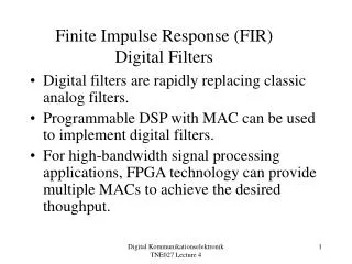
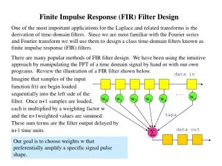
Digital IIR Filters • Infinite Impulse Response (IIR) filter has impulse response of infinite duration, e.g. • How to implement the IIR filter by computer? Let x[k] be the input signal and y[k] the output signal, Z Recursively compute output y[n], n ≥ 0, given y[-1] andx[n]
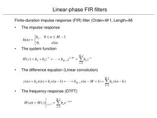
Difference equation Recursive computation needs y[-1] and y[-2] For the filter to be LTI,y[-1] = 0 and y[-2] = 0 Transfer function Assumes LTI system Block diagram representation Second-order filter section (a.k.a. biquad) with 2 poles and 0 zeros x[n] y[n] UnitDelay 1/2 y[n-1] UnitDelay 1/8 y[n-2] Different Filter Representations Poles at –0.183 and +0.683
Discrete-Time IIR Biquad • Two poles, and zero, one, or two zeros • Overall transfer function Real a1, a2 : poles are conjugate symmetric ( j ) or real Real b0, b1, b2 : zeros are conjugate symmetric or real v[n] x[n] b0 y[n] UnitDelay a1 b1 v[n-1] Biquad is short for biquadratic− transfer function is ratio of two quadratic polynomials UnitDelay v[n-2] a2 b2
Discrete-Time IIR Filter Design • Biquad w/ zeros z0 and z1and poles p0 and p1 Magnitude response |a – b| is distance betweencomplex numbers a and b |ej– p0| is distance from pointon unit circle ej and pole location p0 • When poles and zeros are separated in angle Poles near unit circle indicate filter’s passband(s) Zeros on/near unit circle indicate stopband(s)
Im(z) Im(z) Im(z) O O X X X O Re(z) Re(z) Re(z) O X X X O O Discrete-Time IIR Biquad Examples • Transfer function • When transfer function coefficients are real-valued Poles (X) are conjugate symmetric or real-valued Zeros (O) are conjugate symmetric or real-valued • Filters below have what magnitude responses? lowpasshighpass bandpass bandstop allpass notch? Zeros are on the unit circle Poles have radius r Zeros have radius 1/r
A Direct Form IIR Realization • IIR filters having rational transfer functions • Direct form realization Dot product of vector of N +1coefficients and vector of currentinput and previous N inputs (FIR section) Dot product of vector of M coefficients and vector of previous M outputs (“FIR” filtering of previous output values) Computation: M + N + 1 multiply-accumulates (MACs) Memory: M + N words for previous inputs/outputs andM + N + 1 words for coefficients
x[n] y[n] b0 UnitDelay UnitDelay a1 b1 x[n-1] y[n-1] UnitDelay UnitDelay aM a2 bN b2 x[n-2] y[n-2] Feed-forward Feedback UnitDelay UnitDelay x[n-N] y[n-M] Filter Structure As a Block Diagram Full Precision Wordlength of y[0] is 2 words. Wordlength of y[n] increases with n for n > 0. M and N may be different
Yet Another Direct Form IIR • Rearrange transfer function to be cascade of an all-pole IIR filter followed by an FIR filter Here, v[n] is the output of an all-pole filter applied to x[n]: • Implementation complexity (assuming MN) Computation: M + N + 1 MACs Memory: M double words for past values of v[n] andM + N + 1 words for coefficients
v[n] x[n] b0 y[n] UnitDelay a1 b1 v[n-1] UnitDelay v[n-2] a2 b2 Feed-forward Feedback UnitDelay v[n-M] aM bN Filter Structure As Block Diagram Full Precision Wordlength of y[0] is2 words and wordlength of v[0] is 1 word. Wordlength of v[n] and y[n]increases with n. M and N may be different M=2 yields a biquad
Demonstrations • Signal Processing First, PEZ Pole Zero Plotter (pezdemo) • DSP First demonstrations, Chapter 8 IIR Filtering Tutorial (Link) Connection Betweeen the Z and Frequency Domains (Link) Time/Frequency/Z Domain Movies for IIR Filters (Link) For username/password help link link link
Review Stability • A discrete-time LTI system is bounded-input bounded-output (BIBO) stable if for any bounded input x[n] such that | x[n] | B1 < , then the filter response y[n] is also bounded | y[n] | B2 < • Proposition: A discrete-time filter with an impulse response of h[n] is BIBO stable if and only if Every finite impulse response LTI system (even after implementation) is BIBO stable A causal infinite impulse response LTI system is BIBO stable if and only if its poles lie inside the unit circle
Review BIBO Stability • Rule #1: For a causal sequence, poles are inside the unit circle (applies to z-transform functions that are ratios of two polynomials) OR • Rule #2: Unit circle is in the region of convergence. (In continuous-time, imaginary axis would be in region of convergence of Laplace transform.) • Example: Stable if |a| < 1 by rule #1 or equivalently Stable if |a| < 1 by rule #2 because |z|>|a| and |a|<1 pole at z=a
Z and Laplace Transforms • Transform difference/differential equations into algebraic equations that are easier to solve • Are complex-valued functions of a complex frequency variable Laplace: s = + j 2 f Z: z = rej • Transform kernels are complex exponentials: eigenfunctions of linear time-invariant systems Laplace: e–s t = e– t –j 2 f t = e – t e– j 2 f t Z: z –n = (rej) –n= r – ne– jn dampening factor oscillation term
f[n] H(z) y[n] Z Laplace H(s) Z and Laplace Transforms • No unique mapping from Z to Laplace domain or from Laplace to Z domain Mapping one complex domain to another is not unique • One possible mapping is impulse invariance Make impulse response of a discrete-time linear time-invariant (LTI) system be a sampled version of the impulse response for the continuous-time LTI system
Im{z} 1 Re{z} Impulse Invariance Mapping • Mapping is z = e s T where T is sampling time Ts Im{s} 1 Let fs = 1 Hz Re{s} -1 1 -1 Poles: s = -1 j z = 0.198 j 0.31 (T = 1 s)Zeros:s = 1 j z = 1.469 j 2.287 (T = 1 s) lowpass, highpass bandpass, bandstop allpass or notch?
Continuous-Time IIR Biquad • Second-order filter section with 2 poles & 0-2 zeros Transfer function is a ratio of two real-valued polynomials Poles and zeros occur in conjugate symmetric pairs • Quality factor: technology independent measure of sensitivity of pole locations to perturbations For an analog biquad with poles at a ±jb, where a < 0, Real poles: b = 0 so Q = ½ (exponential decay response) Imaginary poles: a = 0 so Q = (oscillatory response)
Continuous-Time IIR Biquad • Impulse response with biquad with poles a ±jb with a < 0 but no zeroes: Pure sinusoid when a = 0 and pure decay when b = 0 • Breadboard implementation Consider a single pole at –1/(R C). With 1% tolerance on breadboard R and C values, tolerance of pole location is 2% How many decimal digits correspond to 2% tolerance? How many bits correspond to 2% tolerance? Maximum quality factor is about 25 for implementation of analog filters using breadboard resistors and capacitors. Switched capacitor filters: Qmax 40 (tolerance 0.2%) Integrated circuit implementations can achieve Qmax 80
Discrete-Time IIR Biquad • For poles at a ±jb = r e ± j , where is the pole radius (r < 1 for stability), with y = –2 a: Real poles: b = 0 and 1 < a < 1, so r = |a| and y = 2 a and Q = ½ (impulse response is C0an u[n] + C1n an u[n]) Poles on unit circle: r = 1 so Q = (oscillatory response) Imaginary poles:a = 0 sor = |b| and y = 0, and 16-bit fixed-point digital signal processors with 40-bit accumulators: Qmax 40 Filter design programs often use r as approximation of quality factor
IIR Filter Implementation • Same approach in discrete and continuous time • Classical IIR filter designs Filter of order n will have n/2 conjugate roots if n is even or one real root and (n-1)/2 conjugate roots if n is odd Response is very sensitive to perturbations in pole locations • Rule-of-thumb for implementing IIR filter Decompose IIR filter into second-order sections (biquads) Cascade biquads from input to output in order of ascending quality factors For each pair of conjugate symmetric poles in a biquad, conjugate zeroes should be chosen as those closest in Euclidean distance to the conjugate poles
Classical IIR Filter Design • Classical IIR filter designs differ in the shape of their magnitude responses Butterworth: monotonically decreases in passband and stopband (no ripple) Chebyshev type I: monotonically decreases in passband but has ripples in the stopband Chebyshev type II: has ripples in passband but monotonically decreases in the stopband Elliptic: has ripples in passband and stopband • Classical IIR filters have poles and zeros, except Continuous-time lowpass Butterworth filters only have poles • Classical filters have biquads with high Q factors
Analog IIR Filter Optimization • Start with an existing (e.g. classical) filter design • IIR filter optimization packages from UT Austin (in Matlab) simultaneously optimize Magnitude response Linear phase in passband Peak overshoot in step response Quality factors
Elliptic Elliptic Optimized Optimized Analog IIR Filter Optimization • Analog lowpass IIR filter design specification dpass= 0.21 at wpass= 20 rad/s and dstop= 0.31 at wstop= 30 rad/s Minimized deviation from linear phase in passband Minimized peak overshoot in step response Maximum quality factor per second-order section is 10 Linearized phase in passband Minimized peak overshoot optimized elliptic
MATLAB Demos Using fdatool #1 • Filter design/analysis • Lowpass filter design specification (all demos) fpass = 9600 Hz fstop = 12000 Hz fsampling = 48000 Hz Apass = 1 dB Astop = 80 dB • Under analysis menu Show magnitude response • FIR filter – equiripple Also called Remez Exchange or Parks-McClellan design Minimum order is 50 Change Wstop to 80 Order 100 gives Astop 100 dB Order 200 gives Astop 175 dB Order 300 does not converge –how to get higher order filter? • FIR filter – Kaiser window Minimum order 101 meets spec
MATLAB Demos Using fdatool #2 • IIR filter – elliptic Use second-order sections Filter order of 8 meets spec Achieved Astop of ~80 dB Poles/zeros separated in angle • Zeros on or near unit circle indicate stopband • Poles near unit circle indicate passband • Two poles very close to unit circle • IIR filter – elliptic Use second-order sections Increase filter order to 9 Eight complex symmetric poles and one real pole: Same observations on left
MATLAB Demos Using fdatool #3 • IIR filter – elliptic Use second-order sections Increase filter order to 20 Two poles very close to unit circle but BIBO stable Use single section (Edit menu) • Oscillation frequency ~9 kHz appears in passband • BIBO unstable: two pairs of poles outside unit circle IIR filter design algorithms return poles-zeroes-gain (PZK format):Impact on response when expanding polynomials in transfer function from factored to unfactored form
MATLAB Demos Using fdatool #4 • IIR filter - constrained least pth-norm design Use second-order sections Limit pole radii ≤ 0.95 Increase weighting in stopband (Wstop) to 10 Filter order 8 does not meet stopband specification Filter order 10 does meet stopband specification Filter order might increase but worth it for more robust implementation
Conclusion (1) For same piecewise constant magnitude specification(2) Algorithm to estimate minimum order for Parks-McClellan algorithm by Kaiser may be off by 10%. Search for minimum order is often needed.(3) Algorithms can tune design to implementation target to minimize risk
Conclusion • Choice of IIR filter structure matters for both analysis and implementation • Keep roots computed by filter design algorithms Polynomial deflation (rooting) reliable in floating-point Polynomial inflation (expansion) may degrade roots • More than 20 IIR filter structures in use Direct forms and cascade of biquads are very common choices • Direct form IIR structures expand zeros and poles May become unstable for large order filters (order > 12) due to degradation in pole locations from polynomial expansion
Conclusion • Cascade of biquads (second-order sections) Only poles and zeros of second-order sections expanded Biquads placed in order of ascending quality factors Optimal ordering of biquads requires exhaustive search • When filter order is fixed, there exists no solution, one solution or an infinite number of solutions • Minimum order design not always most efficient Efficiency depends on target implementation Consider power-of-two coefficient design Efficient designs may require search of infinite design space