Download
1 / 14
140 likes | 579 Views
The Demand for Money. Theories and Evidence. The Demand for Money. So far we have considered the money supply and how a central bank goes about changing it. Where does money demand come from?

E N D
The Demand for Money Theories and Evidence
The Demand for Money • So far we have considered the money supply and how a central bank goes about changing it. • Where does money demand come from? • Understanding the demand for money will allow us to examine the links between monetary policy, inflation, and unemployment. • The quantity of money circulating around the economy and the interest rate at which it circulates are determined by both money supply and money demand.
The Quantity Theory of Money • How much money would you need to purchase the economy’s annual output of goods and services? • Suppose GDP (P*Y) was $14 trillion. • Would you need a money supply of $14 trillion to buy all this output over the course of a year? • No! Each dollar is used multiple times. You would need considerably less M than P*Y. • Velocity is defined as the number of times a dollar bill changes hands over the course of a year in an economy. • It tells us the turnover rate for money in the economy. • Equation of Exchange: M*V ≡ P*Y • The total money supply multiplied by the number of times this money changes hands must be equal to nominal income (or nominal GDP) • Total expenditure (M*V) = Total production (P*Y) • Everything produced is consumed
The Quantity Theory of Money • When the money market is in equilibrium, Md = Ms = M. • The quantity theory of money can be re-written as: • Md = (1/V)*PY • Md = k*PY (k = 1/V = constant if V is a constant) • The demand for money is solely a function of nominal GDP • Money demand is not directly affected by interest rates.
The Liquidity Preference Theory of Money • As seen, velocity cannot be accurately treated as a constant. • If velocity can change, then the link between prices and money is muddled. • J.M. Keynes postulated that individuals hold money for three reasons: • Transactions Motive You need money to buy things • Precautionary Motive You might need money on hand for an unexpected purchase • Speculative Motive You hold your wealth as money (as opposed to bonds) to store value • The biggest innovation was to identify a link between money and interest rates (an inverse relationship.)
The Liquidity Preference Function • What people really care about is the purchasing power of their money • If prices rise, then the real value of money falls. • Want to look at the demand for real money balances • Md/P = f(i,Y) • Real money demand is a decreasing function of nominal interest rates • Real money demand is an increasing function of real income. • Recall that M*V ≡ P*Y • V = P*Y/M • P/Md = 1/f(i,Y) • V = Y/f(i,Y) when the market for money is in equilibrium. • As i↑, f(i,Y)↓, and V↑ Velocity is not constant!
The Transactions Motive for Holding Money • Suppose you earn $3000 per month and consume $100 per day. • We’ll assume 30 day months and a constant rate of consumption over this period. • Case 1: You hold the entire $3000 in cash to carry out your transactions. • You have $3000 at the beginning of the month and $0 at the end. • Your average cash balance is $1500. • Your annual income (P*Y) $36,000 and your holdings of money (M) average $1500. • V = PY/M = 36,000/1500 = 24 • Case 2: You hold $1500 in cash and buy $1500 in bonds at the beginning of each month • After 15 days, you sell your bonds and use the principal ($1500) to make your purchases, keeping any earned interest for yourself. • Your average cash balance is now $750 (1500 at day 1, 0 at day 15, 1500 at day 16, 0 at day 30: (1500+0+1500+0)/4 = 750. • V = PY/M = 36,000/750 = 48 • If i = 1% per month, you also earned (i/2)*1500 = .005*1500 = $7.50
Two Cases Cash on Hand Cash on Hand 3000 1500 1500 750 Time 0 0 2 1 Time 2 1.5 ¼ ½ 1 ½
The Transactions Motive for Holding Money • Case 3: Now suppose you hold $500 in cash and buy $2500 in bonds. • Every 5 days (1/6th month) you run out of cash and have to sell $500 worth of bonds to make your purchases. • Your average cash holdings over the course of the month is M = $250. • V = 36,000/250 = 144 • At 1% monthly interest, you earn (1/6*1%*$2500)+(1/6*1%*$2000)+…+(1/6*1%*500) = $12.50 • As your average cash balance shrinks, both velocity and the interest earned on bonds increases. • So why not hold the smallest amount of cash possible? • Transactions costs of bonds! • Brokerage fees • Time costs • As interest rates rise, people want to hold smaller average cash balances, causing money demand to fall and velocity to rise. • As transactions costs of bonds rise, people want to hold more money at any given point, causing money demand to rise and velocity to fall.
The Speculative Motive • A weakness of Keynes’ original analysis of the speculative motive is that it has a knife edge solution • If the return on bonds is higher, then all speculation is in bonds. If the return on money is higher, then all speculation is in money. • Only when the two assets have identical returns (an uncommon occurrence) will people hold money and bonds for speculative purposes. • James Tobin offered a refinement in 1958 by arguing that people care about both expected returns and risk. • Money has a certain nominal return: zero • Bonds have more volatile returns that may in fact be negative. • Through carrying a diversified portfolio of money and bonds, the overall risk of the portfolio may be minimized relative to expected returns. • However, it is not clear that money offers any greater diversification benefits than near risk-free bonds such as U.S. treasury bills. • No speculative motive for holding money?
Friedman’s Modern Quantity Theory of Money • Milton Friedman built upon Keynes’ idea and introduced his own model of the demand for money: • Real money demand is a function of… • Permanent income (YP), expected average income over the course of one’s life. (+) • The excess return on bonds over money (-) • The excess return on equities over money (-) • The rate at which money loses purchasing power. Can also be thought of as the excess return on goods over money. (-)
Conclusions of Friedman’s Refinement • Includes alternative assets to money • Views money and goods as substitutes • While the expected return on money is not a constant, the excess return on bonds (rb – rm) is assumed to be a constant. • Thus, interest rates (because they cause the returns on all assets to rise by the same proportion) will not affect money demand. • Therefore, the demand for money is predictable a direct function of permanent income. • Thus, Velocity is predictable and stable! • MV = PY Money is the primary determinant of aggregate spending.
Empirical Evidence • Money and Interest Rates • Money demand does appear to be sensitive to interest rates • In the extreme case, money demand is so sensitive to interest rates that it is a flat curve at the current rate. • Known as a liquidity trap, since monetary policy cannot affect interest rates in this case. • Very little evidence that money demand hits a liquidity trap at interest rates above zero. • When nominal interest rates approach zero, we can fall into such a trap (see Japan). • The Money Demand function is variable and unpredictable in Keynes’ model, but stable in Friedman’s model • Before 1970, Md was fairly stable. • Since 1970, Md has been much less stable due to the rapid pace of financial innovation. • Greater instability in Md makes monetary policy harder to control and less predictable.