Binomial heaps, Fibonacci heaps, and applications

Binomial heaps,Fibonacci heaps,and applications

Binomial trees B0 B1 Bi B(i-1) B(i-1)

Binomial trees Bi . . . . . . B0 B(i-1) B(i-2) B1

Properties of binomial trees 1) | Bk | = 2k 2) degree(root(Bk))= k 3) depth(Bk)= k ==> The degree and depth of a binomial tree with at most n nodes is at most log(n). Define the rank of Bk to be k

5 1 5 2 5 5 6 6 8 9 10 Binomial heaps (def) A collection of binomial trees at most one of every rank. Items at the nodes, heap ordered. Possible rep: Doubly link roots and children of every nodes. Parent pointers needed for delete.

5 1 5 5 2 6 6 4 10 6 8 9 9 11 9 10 Binomial heaps (operations) Operations are defined via a basic operation, called linking, of binomial trees: Produce a Bk from two Bk-1, keep heap order.

Binomial heaps (ops cont.) Basic operation is meld(h1,h2): Like addition of binary numbers. B5 B4 B2 B1 h1: B4 B3 B1 B0 + h2: B4 B3 B0 B5 B4 B2

Binomial heaps (ops cont.) Findmin(h): obvious Insert(x,h) : meld a new heap with a single B0 containing x, with h deletemin(h) : Chop off the minimal root. Meld the subtrees with h. Update minimum pointer if needed. delete(x,h) : Bubble up and continue like delete-min decrease-key(x,h,) : Bubble up, update min ptr if needed All operations take O(log n) time on the worst case, except find-min(h) that takes O(1) time.

Amortized analysis We are interested in the worst case running time of a sequenceof operations. Example: binary counter single operation -- increment 00000 00001 00010 00011 00100 00101

Amortized analysis (Cont.) On the worst case increment takes O(k). k = #digits What is the complexity of a sequence of increments (on the worst case) ? Define a potential of the counter:  (c) = ? Amortized(increment) = actual(increment) + 

+ Amortized analysis (Cont.) Amortized(increment1) = actual(increment1) + 1-0 Amortized(increment2) = actual(increment2) + 2-1 … … Amortized(incrementn) = actual(incrementn) + n-(n-1) iAmortized(incrementi) = iactual(incrementi) + n-0 iAmortized(incrementi) iactual(incrementi) if n-0  0

Amortized analysis (Cont.) Define a potential of the counter:  (c) = #(ones) Amortized(increment) = actual(increment) +  Amortized(increment) = 1+ #(1 => 0) + 1 - #(1 => 0) = O(1) ==> Sequence of n increments takes O(n) time

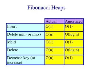
Binomial heaps - amortized ana.  (collection of heaps) = #(trees) Amortized cost of insert O(1) Amortized cost of other operations still O(log n)

Binomial heaps + lazy meld Allow more than one tree of each rank. • Meld (h1,h2) : • Concatenate the lists of binomial trees. • Update the minimum pointer to be the smaller of the minimums O(1) worst case and amortized.

Binomial heaps + lazy meld As long as we do not do a delete-min our heaps are just doubly linked lists: 9 11 4 6 9 5 Delete-min : Chop off the minimum root, add its children to the list of trees. Successive linking: Traverse the forest keep linking trees of the same rank, maintain a pointer to the minimum root.

Binomial heaps + lazy meld Possible implementation of delete-min is using an array indexed by rank to keep at most one binomial tree of each rank that we already traversed. Once we encounter a second tree of some rank we link them and keep linking until we do not have two trees of the same rank. We record the resulting tree in the array Amortized(delete-min) = = (#(trees at the end) + #links + max-rank) - #links  (2log(n) + #links) - #links = O(log(n))

Binomial heaps + lazy delete Allow more than one tree of each rank. Meld (h1,h2), Insert(x,h) -- as before Delete(x,h) : simply mark x as deleted. Deletemin(h) : y = findmin(h) ; delete(y,h) How do we do findmin ?

Binomial heaps + lazy delete Traverse the trees top down purging deleted nodes and stopping at each non-deleted node Do successive linking on the forest you obtain.

Binomial heaps + lazy delete

Binomial heaps + lazy delete (ana.) Modify the potential a little:  (collection of heaps) = #(trees) + #(deleted nodes) Insert, meld, delete : O(1) delete-min : like find-min What is the amortized cost of find-min ?

Binomial heaps + lazy delete (ana.) What is the amortized cost of find-min ? amortized(find-min) = amortized(purging) + amortized(successive linking + scan of undeleted nodes) We saw that: amortized(successive linking) = O(log(n)) Amortized(purge) = actual(purge) + (purge) Actual(purge) = #(nodes purged) + #(new trees) (purge) = #(new trees)- #(nodes purged) So, amortized(find-min) = O(log(n) + #(new trees) )

Binomial heaps + lazy delete (ana.) How many new trees are created by the purging step ? Let p = #(nodes purged), n = total #(nodes) Then #(new trees) = O( p*(log(n/p)+ 1) ) So, amortized(find-min) = O( p*(log(n/p)+ 1) ) Proof. Suppose the i-th purged node, 1  i  p, had ki undeleted children. One of them has degree at least ki-1. Therefore in its subtree there are at least 2(ki-1) nodes.

Binomial heaps + lazy delete (ana.) Proof (cont). How large can k1+k2+ . . . +kp be such that i=1 2(ki-1)  n ? Make all ki equal log(n/p) + 1, then i ki = p*(log(n/p)+ 1) p

Application: The round robin algorithm of Cheriton and Tarjan (76) for MST We shall use a Union-Find data structure. The union find problem is where we want to maintain a collection of disjoint sets under the operations 1) S=Union(S1,S2) 2) S=find(x) Can do it in O(1) amortized time for union and O((k,n)) amortized time for find, where k is the # of finds, and n is the number of items (assuming k ≥ n).

A greedy algorithm for MST Start with a forest where each tree is a singleton. Repeat the following step until there is only one tree in the forest: Pick T  F, pick a minimum cost edge e connecting a vertex of T to a vertex in T’, add e to the forest (merge T and T’ to one tree) Prim’s algorithm: picks always the same T Kruskal’s algorithm: picks the lightest edge out of F

Cheriton & Tarjan’s ideas Keep the trees in a queue, pick the first tree, T, in the queue, pick the lightest edge e connecting it to another tree T’. Remove T’ from the queue, connect T and T’ with e. Add the resulting tree to the end of the queue.

Cheriton & Tarjan (cont.) T’ T e T’ T e

Cheriton & Tarjan (implementation) The vertices of each tree T will be a set in a Union-Find data structure. Denote it also by T Edges with one endpoint in T are stored in a heap data structure. Denoted by h(T). We use binomial queues with lazy meld and deletion. Find e by doing find-min on h(T). Let e=(v,w). Find T’ by doing find(w). Then create the new tree by T’’= union(T,T’) and h(T’’) = meld(h(T),h(T’))

Cheriton & Tarjan (implementation) Note: The meld implicitly delete edges. Every edge in h(T) with both endpoints in T is considered as “marked deleted”. We never explicitly delete edges! We can determine whether an edge is deleted or not by two find operations.

Cheriton & Tarjan (analysis) • Assume for the moment that find costs O(1) time. • Then we can determine whether a node is marked deleted in O(1) time, and our analysis is still valid. • So, we have • at most 2m implicit delete operations that cost O(m). • at most n find operations that cost O(n). • at most n meld and union operations that cost O(n). • at most n find-min operations. The complexity of these find-min operations dominates the complexity of the algorithm.

Cheriton & Tarjan (analysis) Let mi be the number of edges in the heap at the i-th iteration. Let pi be the number of deleted edges purged from the heap at the find-min performed by the i-th iteration. So, we proved that the i-th find-min costs O(pi*(log(mi / pi)+ 1) ). We want to bound the sum of these expressions. We will bound i mi first.

Cheriton & Tarjan (analysis) Divide the iterations into passes as follows. Pass 1 is when we remove the original singleton trees from the queue. Pass i is when we remove trees added to the queue at pass i-1. What is the size of a tree removed from the queue at pass j ? At least 2j . (Prove by induction) So how many passes are there ? At most log(n)

Cheriton & Tarjan (analysis) An edge can occur in at most two heaps of trees in one pass. So i mi  2m log(n) Recall we want to bound O(i pi*(log(mi / pi)+ 1) ). 1) Consider all find-mins such that pi  mi / log2(n): O(i pi*(log(mi / pi)+ 1) ) = O(i pi log log(n)) = O(m loglog(n)) 2) Consider all find-mins such that pi  mi / log2(n): O(i pi*(log(mi / pi)+ 1) ) = O(i (mi / log2(n))log(mi)) = O(m)

Cheriton & Tarjan (analysis) We obtained a time bound of O(m loglog(n)) under the assumption that find takes O(1) time. But if you amortize the cost of the finds on O(m loglog(n)) operations then the cost per find is really (m loglog(n),n) = O(1)

Fibonacci heaps (Fredman & Tarjan 84) Want to do decrease-key(x,h,) faster than delete+insert. Ideally in O(1) time. Why ?

Dijkstra’s shortest path algorithm Let G = (V,E) be a weighted (weights are non-negative) undirected graph, let s  V. Want to find the distance (length of the shortest path), d(s,v) from s to every other vertex. 3 3 s 2 1 3 2

Dijkstra’s shortest path algorithm • Dijkstra: Maintain an upper bound d(v) on d(s,v). • Every vertex is either scanned, labeled, or unlabeled. • Initially: d(s) = 0 and d(v) =  for every v  s. • s is labeled and all others are unlabeled. • Pick a labeled vertex with d(v) minimum. Make v scanned. • For every edge (v,w) if d(v) + w(v,w) < d(w) then • 1) d(w) := d(v) + w(v,w) • 2) label w if it is not labeled already

Dijkstra’s shortest path algorithm (implementation) Maintain the labeled vertices in a heap, using d(v) as the key of v. We perform n delete-min operations and n insert operations on the heap. O(n log(n)) For each edge we may perform a decrease-key. With regular heaps O(m log (n)). But if you can do decrease-key in O(1) time then you can implement Dijkstra’s algorithm to run in O(n log(n) + m) time !

Back to Fibonacci heaps Suggested implementation for decrease-key(x,h,): If x with its new key is smaller than its parent, cut the subtree rooted at x and add it to the forest. Update the minimum pointer if necessary.

5 2 5 3 5 1 5 5 5 2 5 5 9 8 6 10 9 8 6 6 6 10

Decrease-key (cont.) Does it work ? Obs1: Trees need not be binomial trees any more.. Do we need the trees to be binomial ? Where have we used it ? In the analysis of delete-min we used the fact that at most log(n) new trees are added to the forest. This was obvious since trees were binomial and contained at most n nodes.

2 9 5 3 6 5 6 Decrease-key (cont.) Such trees are now legitimate. So our analysis breaks down.

Fibonacci heaps (cont.) We shall allow non-binomial trees, but will keep the degrees logarithmic in the number of nodes. Rank of a tree = degree of the root. Delete-min: do successive linking of trees of the same rank and update the minimum pointer as before. Insert and meld also work as before.

Fibonacci heaps (cont.) Decrease-key (x,h,): indeed cuts the subtree rooted by x if necessary as we showed. in addition we maintain a mark bit for every node. When we cut the subtree rooted by x we check the mark bit of p(x). If it is set then we cut p(x) too. We continue this way until either we reach an unmarked node in which case we mark it, or we reach the root. This mechanism is called cascading cuts.

9 5 7 4 2 20 16 6 14 8 11 12 15 2 4 20 5 8 11 9 6 14 10 16 12 15

Fibonacci heaps (delete) Delete(x,h) : Cut the subtree rooted at x and then proceed with cascading cuts as for decrease key. Chop off x from being the root of its subtree and add the subtrees rooted by its children to the forest If x is the minimum node do successive linking

Fibonacci heaps (analysis) Want everything to be O(1) time except for delete and delete-min. ==> cascading cuts should pay for themselves  (collection of heaps) = #(trees) + 2#(marked nodes) Actual(decrease-key) = O(1) + #(cascading cuts) (decrease-key) = O(1) - #(cascading cuts) ==> amortized(decrease-key) = O(1) !

Fibonacci heaps (analysis) What about delete and delete-min ? Cascading cuts and successive linking will pay for themselves. The only question is what is the maximum degree of a node ? How many trees are being added into the forest when we chop off a root ?

x Proof: When the i-th node was linked it must have had at least i-1 children. Since then it could have lost at most one. Fibonacci heaps (analysis) Lemma 1 : Let x be any node in an F-heap. Arrange the children of x in the order they were linked to x, from earliest to latest. Then the i-th child of x has rank at least i-2. 2 1

Binomial heaps, Fibonacci heaps, and applications