Sorting Algorithms : Topic Overview

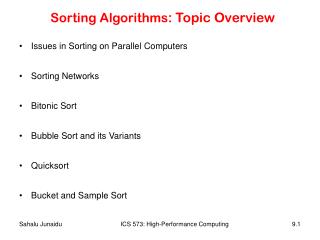
1. Sorting Algorithms: Topic Overview • Issues in Sorting on Parallel Computers • Sorting Networks • Bitonic Sort • Bubble Sort and its Variants • Quicksort • Bucket and Sample Sort ICS 573: High-Performance Computing

2. Sorting: Overview • One of the most commonly used and well-studied kernels. • many algorithms require sorted data for easier manipulation • Sorting algorithms • internal • external • comparison-based: based on compare-exchange • noncomparison-based: based on elements’ properties like their binary representation or their distribution • Lower bound complexity classes to sort n numbers: • Comparison-based: Θ(nlog n). • Noncomparison-based: Θ(n). • We focus here on comparison-based sorting algorithms. ICS 573: High-Performance Computing

3. Issues in Sorting on Parallel Computers • Where are the input and output lists stored? • We assume that the input and output lists are distributed. • Input specification • Each processor has n/p elements • An ordering of the processors • Output specification • Each processor will get n/p consecutive elements of the final sorted array. • The “chunk” is determined by the processor ordering. • Variations • Unequal number of elements on output. • In general, this is not a good idea and it may require a shift to obtain the equal size distribution. ICS 573: High-Performance Computing

4. Parallel Compare-Exchange Operation • Comparison becomes more complicated when elements reside on different processes • One element per process: ICS 573: High-Performance Computing

5. Parallel Compare-Split Operation • The compare-exchange communication cost is ts + tw. • Assuming bidirectional channels • Delivers poor performance. Why? • More than one element per process: compare-split operation. • Assume each of two processes has n/pelements. • After the compare-split operation, • the smaller n/p elements are at process Pi and • the larger n/p elements at Pi, where i < j. • The compare-split communication cost is ts+ twn/p. • Assuming that the two partial lists were initially sorted. ICS 573: High-Performance Computing

6. Parallel Compare-Split Operation ICS 573: High-Performance Computing

7. Sorting Networks • Key Idea: • Perform many comparisons in parallel. • Key Elements: • Comparators: • Consist of two-input, two-output wires • Take two elements on the input wires and outputs them in sorted order in the output wires. • Network architecture: • The arrangement of the comparators into interconnected comparator columns • similar to multi-stage networks • Many sorting networks have been developed. • Bitonic sorting network with Θ(log2(n)) columns of comparators. ICS 573: High-Performance Computing

8. Sorting Networks: Comparators • A comparator is a device with two inputs x and y and two outputs x' and y'. • For an increasing comparator, x' = min{x,y} and y' = max{x,y}; • For an decreasing comparator, x' = max{x,y} and y' = min{x,y}; • We denote an increasing comparator byand a decreasing comparator by Ө. • Consists of a series of columns each with comparators connected in parallel. • The depth of a network is the number of columns it contains. ICS 573: High-Performance Computing

9. Sorting Networks: Comparators ICS 573: High-Performance Computing

10. Sorting Networks: Architecture ICS 573: High-Performance Computing

11. Bitonic Sort • Bitonic sorting depends on rearranging a bitonic sequence into a sorted sequence. • Uses a bitonic sorting network to sort n elements in Θ(log2n) time. • A bitonic sequence <a0, a1, ..., an-1> is such that either • there exists an index i, 0 ≤ i ≤ n - 1, such that • <a0, ..., ai > is monotonically increasing and • <ai +1, ..., an-1> is monotonically decreasing, or • there exists a cyclic shift of indices so that (1) is satisfied. • Example bitonic sequences: • 1,2,4,7,6,0 • 8,9,2,1,0,4 because it is a cyclic shift of 0,4,8,9,2,1. ICS 573: High-Performance Computing

12. Sorting a Bitonic Sequence • Let s=a0,a1,…,an-1 be a bitonic sequence such that • a0 ≤ a1 ≤ ··· ≤ an/2-1 and • an/2 ≥an/2+1 ≥ ··· ≥ an-1. • Consider the following subsequences of s: s1 = min{a0,an/2},min{a1,an/2+1},…,min{an/2-1,an-1} s2 = max{a0,an/2},max{a1,an/2+1},…,max{an/2-1,an-1} • Dividing a bitonic sequence into two subsequences as above is called a bitonic split • Note that s1 and s2 are both bitonic and each element of s1 is less than every element in s2. • Apply bitonic split recursively on s1 and s2 to get the sorted sequence. • Sorting a bitonic sequence this way is called bitonic merge • How many bitonic splits are required to sort a bitonic sequence? ICS 573: High-Performance Computing

13. Example: Bitonic Sort ICS 573: High-Performance Computing

14. Bitonic Merging Network (BMN) • BMN: a network of comparators used to implement the bitonic merge algorithm. • BMN contains log n columns each containing n/2 comparators • Each column performs one step of the bitonic merge. • BMN takes as input the bitonic sequence and outputs the sequence in sorted order. • We denote a bitonic merging network with n inputs by BM[n]. • Replacing the  comparators by Ө comparators results in a decreasing output sequence; such a network is denoted by ӨBM[n]. ICS 573: High-Performance Computing

15. Example: Using a Bitonic Merging Network ICS 573: High-Performance Computing

16. Sorting Unordered Elements • Sorting can be achieved by repeatedly merging bitonic sequences of increasing lengths • Resulting in a single bitonic sequence from the given sequence. • A sequence of length 2 is a bitonic sequence. Why? • A bitonic sequence of length 4 can be built by sorting the first two elements using BM[2] and next two, using ӨBM[2]. • This process can be repeated to generate larger bitonic sequences. • The algorithm embodied in this process is called Bitonic Sort and the network is called a Bitonic Sorting Network (BSN). ICS 573: High-Performance Computing

17. Sorting Unordered Elements Using a BSN ICS 573: High-Performance Computing

18. Details of Sorting Using a BSN ICS 573: High-Performance Computing

19. Complexity of Bitonic Sort • How many stages are there in a BSN for sorting n elements? • What is the depth (# of steps/columns) of the network? • Stage i consists of i columns of n/2 comparators • How many comparators are there? • n/2 log2 n • Thus, a serial implementation of the network would have complexity Θ(n log2 n). ICS 573: High-Performance Computing

20. Bitonic Sort on Parallel Computers • A key aspect of bitonic sort: communication intensive • A proper mapping must take into account the topology of the underlying interconnection network • We discuss mapping to hypercube and mesh topologies • Mapping requirements for good performance • Map wires that perform compare-exchange onto neighboring processes • Map wires that perform compare-exchange more frequently onto neighboring processes • How are wires paired to do compare-exchange in each stage? • Which wires communicate most frequently? • Wires whose labels differ in the ith least-significant bit perform compare-exchange log n – i + 1 times ICS 573: High-Performance Computing

21. Mapping Bitonic Sort to Hypercubes • Case 1: one item per processor. • What is the comparator? • How do the wires get mapped? • Recall that processes whose labels differ in only one bit are neighbors in a hypercube • This provides a direct mapping of wires to processors. All communication is nearest neighbor! • Pairing processes in a d-dimensional hypercube (p=2d): • Consider the steps during the last stage of the algorithm: • Step 1: processes differing in dth bit exchange elements along the dth dimension • Step 2: compare-exchange takes place along (d-1)th dimension • Step i: compare-exchange takes place along (d-(i-1))th dimension ICS 573: High-Performance Computing

22. Mapping Bitonic Sort to Hypercubes ICS 573: High-Performance Computing

23. Communication Pattern of Bitonic Sort on Hypercubes ICS 573: High-Performance Computing

24. Bitonic Sort Algorithm on Hypercubes • Parallel runtime: Tp= Θ(log2 n) ICS 573: High-Performance Computing

25. Mapping Bitonic Sort to Meshes • The connectivity of a mesh is lower than that of a hypercube, so we must expect some overhead in this mapping. • So we map wires such that the most frequent compare-exchange operations occur between neighboring processes. • Some mapping options: • row-major mapping, • row-major snakelike mapping, and • row-major shuffled mapping. • Each process is labeled by the wire that is mapped onto it. • Advantage of row-major shuffled mapping • processes that perform compare-exchange operations reside on square subsections of the mesh. • wires that differ in the ith least-significant bit are mapped onto mesh processes that are communication links away. ICS 573: High-Performance Computing

26. Bitonic Sort on Meshes: Example Mappings ICS 573: High-Performance Computing

27. Mapping Bitonic Sort to Meshes ICS 573: High-Performance Computing

28. Parallel Time of Bitonic Sort on Meshes • Row-major shuffled mapping • wires that differ at the ith least-significant bit are mapped onto mesh processes that are 2(i-1)/2 communication links away. • The total amount of communication performed by each process is: • The total computation performed by each process is Θ(log2n). • The parallel runtime is: ICS 573: High-Performance Computing

29. Block of Elements Per Processor • Each process is assigned a block of n/p elements. • The first step is a local sort of the local block. • Each subsequent compare-exchange operation is replaced by a compare-split operation. • We can effectively view the bitonic network as having (1 + log p)(log p)/2 steps. ICS 573: High-Performance Computing

30. Block of Elements Per Processor: Hypercube • Initially the processes sort their n/p elements (using merge sort) in time Θ((n/p)log(n/p)) • and then perform Θ(log2p)compare-split steps. • The parallel run time of this formulation is ICS 573: High-Performance Computing

31. Block of Elements Per Processor: Mesh • The parallel runtime in this case is given by: ICS 573: High-Performance Computing

32. Bubble Sort and its Variants • We now focus on traditional sorting algorithms. • We’ll investigate whether n processes can be employed to sort a sequence in Θ(log n)time. • Recall that the sequential bubble sort algorithm compares and exchanges adjacent elements. • The complexity of bubble sort is Θ(n2). • Bubble sort is difficult to parallelize since the algorithm has no concurrency. ICS 573: High-Performance Computing

33. Sequential Bubble Sort Algorithm ICS 573: High-Performance Computing

34. Odd-Even Transposition Sort: A Bubble Sort Variant • Odd-Even sort alternates between two phases, called the odd and even phases • Odd phase: compare-exchange elements with odd indices with their right neighbors • Similarly for even phase. • Sequence is sorted after n phases (n is even), each of which requires n/2 compare-exchange operations. • Thus, its sequential complexity is Θ(n2). ICS 573: High-Performance Computing

35. Sequential Odd-Even Sort Algorithm ICS 573: High-Performance Computing

36. Example: Odd-Even Sort Algorithm ICS 573: High-Performance Computing

37. Parallel Odd-Even Transposition • Consider the one item per process case. • There are n iterations, in each iteration, each process does one compare-exchange. • The parallel run time of this formulation is Θ(n). • This is cost optimal with respect to the base serial algorithm but not the optimal one. ICS 573: High-Performance Computing

38. Parallel Odd-Even Transposition ICS 573: High-Performance Computing

39. Parallel Odd-Even Transposition • Consider a block of n/p elements per process. • The first step is a local sort. • Then the processes execute p phases • In each subsequent step, the compare-exchange operation is replaced by the compare-split operation. • The parallel run time of the formulation is ICS 573: High-Performance Computing

40. Shellsort • Shellsort can provide a substantial improvement over odd- even sort. • Moves elements long distances towards their final positions. • Consider sorting n elements using p=2d processes. • Assumptions • Processes are ordered in a logical one-D array, and this ordering defines the global ordering of the sorted sequence • Each process is assigned n/p elements • Two phases of the algorithm: • During the first phase, processes that are far away from each other in the array compare-split their elements. • During the second phase, the algorithm switches to an odd-even transposition sort. • The odd-even phases are performed only as long as the blocks on the processes are changing • Note that elements are moved closer to their final positions in the first phase • Thus the even-odd phases performed may be much smaller than p. ICS 573: High-Performance Computing

41. Parallel Shellsort • Initially, each process sorts its block of n/p elements internally. • Each process is now paired with its corresponding process in the reverse order of the array. • That is, process Pi, where i < p/2, is paired with process Pp-i-1. • A compare-split operation is performed. • The processes are split into two groups of size p/2 each and the process repeated in each group. • Process continues for d steps ICS 573: High-Performance Computing

42. A Phase in Parallel Shellsort ICS 573: High-Performance Computing

43. Complexity of Parallel Shellsort • Each process performs d = log p compare-split operations. • In the second phase, l odd and even phases are performed, each requiring time Θ(n/p). • The parallel run time of the algorithm is: ICS 573: High-Performance Computing

44. Quicksort • Quicksort is one of the most common sequential algorithms due to its • simplicity, • low overhead, and • optimal average complexity. • It is a divide-and-conquer algorithm • Pivot selection • Divide step: partitioning into to subsequences based on the pivot • Conquer step: sort the two subsequence recursively using quicksort ICS 573: High-Performance Computing

45. Sequential Quicksort ICS 573: High-Performance Computing

46. Tracing Quicksort ICS 573: High-Performance Computing

47. Complexity of Quicksort • The performance of quicksort depends critically on the quality of the pivot. • There are many methods for selecting the pivot • A poorly selected pivot leads to worst performance • n2 complexity • A well-selected pivot leads to optimum performance • n log ncomplexity. ICS 573: High-Performance Computing

48. Parallelizing Quicksort • Recursive decomposition provides a natural way of parallelizing quicksort • Execute on a single process, initially • Then assign one of the subproblems to other processes • Limitations of this parallel formulation: • Uses n processes to sort n items • Performs the partitioning step serially • Can we use n processes to partition a list of length n around a pivot in O(1) time? • We present three parallel formulations that perform the partitioning step in parallel: • PRAM formulation • Shared-address space (SAS) formulation • Message-Passing (M-P) formulation ICS 573: High-Performance Computing

49. PRAM Formulation • We assume a CRCW (concurrent read, concurrent write) PRAM with concurrent writes resulting in an arbitrary write succeeding. • The formulation works by creating pools of processes. • Every process is assigned to the same pool initially and has one element. • Each processor attempts to write its element to a common location (for the pool). • Each process tries to read back the location. • If the value read back is greater than the processor's value, it assigns itself to the `left' pool, else, it assigns itself to the `right' pool. • Each pool performs this operation recursively. ICS 573: High-Performance Computing

50. PRAM Formulation: Illustration ICS 573: High-Performance Computing