Download
1 / 35
360 likes | 679 Views
Game Theory II. Definition of Nash Equilibrium. A game has n players. Each player i has a strategy set S i This is his possible actions Each player has a payoff function p I : S ! R

E N D
Definition of Nash Equilibrium • A game has n players. • Each player i has a strategy set Si • This is his possible actions • Each player has a payoff function • pI: S ! R • A strategy ti2 Siis a best response if there is no other strategy in Si that produces a higher payoff, given the opponent’s strategies.
Definition of Nash Equilibrium • A strategy profile is a list (s1, s2, …, sn) of the strategies each player is using. • If each strategy is a best response given the other strategies in the profile, the profile is a Nash equilibrium. • Why is this important? • If we assume players are rational, they will play Nash strategies. • Even less-than-rational play will often converge to Nash in repeated settings.
An Example of a Nash Equilibrium Column a b a 1,2 0,1 Row b 1,0 2,1 (b,a) is a Nash equilibrium. To prove this: Given that column is playing a, row’s best response is b. Given that row is playing b, column’s best response is a.
Finding Nash Equilibria – Dominated Strategies • What to do when it’s not obvious what the equilibrium is? • In some cases, we can eliminate dominated strategies. • These are strategies that are inferior for every opponent action. • In the previous example, row = a is dominated.
Example • A 3x3 example: Column a b c a 73,25 57,42 66,32 Row b 80,26 35,12 32,54 c 28,27 63,31 54,29
Example Column • A 3x3 example: a b c a 73,25 57,42 66,32 Row b 80,26 35,12 32,54 c 28,27 63,31 54,29 c dominates a for the column player
Example Column • A 3x3 example: a b c a 73,25 57,42 66,32 Row b 80,26 35,12 32,54 c 28,27 63,31 54,29 b is then dominated by both a and c for the row player.
Example Column • A 3x3 example: a b c a 73,25 57,42 66,32 Row b 80,26 35,12 32,54 c 28,27 63,31 54,29 Given this, b dominates c for the column player – the column player will always play b.
Example Column • A 3x3 example: a b c a 73,25 57,42 66,32 Row b 80,26 35,12 32,54 c 28,27 63,31 54,29 Since column is playing b, row will prefer c.
Example Column a b c a 73,25 57,42 66,32 Row b 80,26 35,12 32,54 c 28,27 63,31 54,29 We verify that (c,b) is a Nash Equilibrium by observation: If row plays c, b is the best response for column. If column plays b, c is the best response by row.
Example #2 • You try this one: Column a b c a 2,2 1,1 4,0 Row b 1,2 4,1 3,5
Coordination Games • Consider the following problem: • A supplier and a buyer need to decide whether to adopt a new purchasing system. Buyer new old new 20,20 0,0 Supplier old 5,5 0,0 No dominated strategies!
Buyer new old new 20,20 0,0 Supplier old 5,5 0,0 Coordination Games • This game has two Nash equilibria (new,new) and (old,old) • Real-life examples: Beta vs VHS, Mac vs Windows vs Linux, others? • Each player wants to do what the other does • which may be different than what they say they’ll do • How to choose a strategy? Nothing is dominated.
Solving Coordination Games • Coordination games turn out to be an important real-life problem • Technology/policy/strategy adoption, delegation of authority, synchronization • Human agents tend to use “focal points” • Solutions that seem to make “natural sense” • e.g. pick a number between 1 and 10 • Social norms/rules are also used • Driving on the right/left side of the road • These strategies change the structure of the game
Finding Nash Equilibria – Simultaneous Equations • We can also express a game as a set of equations. • Demand for corn is governed by the following equation: • Quantity = 100000(10 – p) • Government price supports say that p must be at least 0.25 (and it can’t be more than 10) • Three farmers can each choose to sell 0-600000 lbs of corn. • What are the Nash equilibria?
Setup • Quantity (q) = q1 + q2 + q3 • Price(p) = a –bq (downward-sloping line) • Farmer 1 is trying to decide a quantity to sell. • Maximize profit = price * quantity • Maximize: pq1 =(a –bq) * q1 • Profit = (a – b(q1 + q2 + q3)) * q1 = = aq1 –bq12 –bq1q2 –bq1q3 Differentiate: Pr’ = a – 2bq1 –bq2 – bq3 To maximize: set this equal to zero.
Setup • So solutions must satisfy • a – b(q2 + q3) – 2bq1 = 0 • So what if q1 = q2 = q3 (everyone ships the same amount?) • Since the game is symmetric, this should be a solution. • a – 4bq1 = 0, a = 4bq1, q1 = a/4b. • q = 3a/4b, p = a/4. Each farmer gets a2 / 16b. • In this problem, a=10, b=1/100000. • Price = $2.50, q1=250000, profit = 625,000 • q1=q2=q3=250000 is a solution. • Price supports not used in this solution.
Setup • What if farmers 2 & 3 send everything they have? • q2 + q3 = 1,200,000 • If farmer 1 then shipped nothing, price would be: • 10 - 1,200,000/100,000 = -2. • But prices can’t fall below $0.25, so they’d be capped there. • Adding quantity would reduce the price, except for supports. • So, farmer 1 should sell all his corn at $0.25, and earn $125,000. • So everyone selling everything at the lowest price (q1 = q2 =q3 = 600,000) is also a Nash equilibrium. • These are the only pure strategy Nash equilibria.
Price-matching Example • Two sellers are offering the same book for sale. • This book costs each seller $25. • The lowest price gets all the customers; if they match, profits are split. • What is the Nash Equilibrium strategy?
Price-matching Example • Suppose the monopoly price of the book is $30. • (price that maximizes profit w/o competition) • Each seller offers a rebate: if you find the book cheaper somewhere else, we’ll sell it to you with double the difference subtracted. • E.g. $30 at store 1, $24 at store 2 – get it for $18 from store 1. • Now what is each seller’s Nash strategy?
Price-matching example • Observation 1: sellers want to have the same price. • Each suffers from giving the rebate. • Profit = p1 – 2(p1 – p2) = -p1 –2p2 • Pr’ = -1. • There is no local maximum. So, to maximize profits, maximize price. • At that point, the rebate 2(p1 – p2) is 0, and p1 is as high as possible. • The 2 makes up for sharing the market.
Cooperative Games and Coalitions • When a group of agents decide to cooperate to improve their payments (for example, adopting a technology), we call them a coalition • Side payments, bribes, intimidation may be used to set up a coalition. • Example: A,B,C are running for class president. The president receives $10, everyone else $0 • Each player’s strategy is to vote for themselves. • A offers B $5 to vote for her – now both A and B are happier and have formed a coalition.
Efficiency • We say that a coalition is efficient if there’s no choice of action that can improve one person’s profit without decreasing another. • Same reasoning as Nash equilibria, market equilibria. • If someone could change their strategy without hurting anyone and improve their payoff, it’s not efficient. • Money is left “on the table” • Example: cake-cutting.
Mixed strategies • Unfortunately, not every game has a pure strategy equilibrium. • Rock-paper-scissors • However, every game has a mixed strategy Nash equilibrium. • Each action is assigned a probability of play. • Player is indifferent between actions, given these probabilities.
Mixed Strategies • In many games (such as coordination games) a player might not have a pure strategy. • Instead, optimizing payoff might require a randomized strategy (also called a mixed strategy) Wife football shopping football 2,1 0,0 Husband shopping 1,2 0,0
Wife football shopping football 2,1 0,0 Husband shopping 1,2 0,0 Strategy Selection If we limit to pure strategies: Husband: U(football) = 0.5 * 2 + 0.5 * 0 = 1 U(shopping) = 0.5 * 0 + 0.5 * 1 = ½ Wife: U(shopping) = 1, U(football) = ½ Problem: this won’t lead to coordination!
Mixed strategy • Instead, each player selects a probability associated with each action • Goal: utility of each action is equal • Players are indifferent to choices at this probability • a=probability husband chooses football • b=probability wife chooses shopping • Since payoffs must be equal, for husband: • b*1=(1-b)*2 b=2/3 • For wife: • a*1=(1-a)*2 = 2/3 • In each case, expected payoff is 2/3 • 2/9 of time go to football, 2/9 shopping, 5/9 miscoordinate • If they could synchronize ahead of time they could do better.
Example: Rock paper scissors Column rock paper scissors 0,0 -1,1 1,-1 rock Row paper 1,-1 0,0 -1,1 scissors -1,1 1,-1 0,0
Setup • Player 1 plays rock with probability pr, scissors with probability ps, paper with probability 1-pr –ps • P2: Utility(rock) = 0*pr + 1*ps – 1(1-pr –ps) = 2 ps + pr -1 • P2: Utility(scissors) = 0*ps + 1*(1 – pr – ps) – 1pr = 1 – 2pr –ps • P2: Utility(paper) = 0*(1-pr –ps)+ 1*pr – 1ps = pr –ps Player 2 wants to choose a probability for each strategy so that the expected payoff for each strategy is the same.
Setup qr(2 ps + pr –1) = qs(1 – 2pr –ps) = (1-qr-qs) (pr –ps) • It turns out (after some algebra) that the optimal mixed strategy is to play each strategy ½ of the time. • Intuition: What if you played rock half the time? Your opponent would then play paper half the time, and you’d lose more often than you won. • So you’d decrease the fraction of times you played rock, until your opponent had no ‘edge’ in guessing what you’ll do.
Repeated games • Many games get played repeatedly • A common strategy for the husband-wife problem is to alternate • This leads to a payoff of 1, 2,1,2,… • 1.5 per week. • Requires initial synchronization, plus trust that partner will go along. • Difference in formulation: we are now thinking of the game as a repeated set of interactions, rather than as a one-shot exchange.
Repeated vs Stage Games • There are two types of multiple-action games: • Stage games: players take a number of actions and then receive a payoff. • Checkers, chess, bidding in an ascending auction • Repeated games: Players repeatedly play a shorter game, receiving payoffs along the way. • Poker, blackjack, rock-paper-scissors, etc
Analyzing Stage Games • Analyzing stage games requires backward induction • We start at the last action, determine what should happen there, and work backwards. • Just like a game tree with extensive form. • Strange things can happen here: • Centipede game • Players alternate – can either cooperate and get $1 from nature or defect and steal $2 from your opponent • Game ends when one player has $100 or one player defects.
Analyzing Repeated Games • Analyzing repeated games requires us to examine the expected utility of different actions. • Assumption: game is played “infinitely often” • Weird endgame effects go away. • Prisoner’s Dilemma again: • In this case, tit-for-tat outperforms defection. • Collusion can also be explained this way. • Short-term cost of undercutting is less than long-run gains from avoiding competition.