Download
1 / 19
200 likes | 436 Views
PSPICE Lecture - AC Circuits. 1. PSPICE – AC Circuits. Reference : (see course web site) PSPICE Assignment #2. Topics to be presented : AC circuits – graphing sinusoidal waveforms using Transient Analysis AC circuits – finding phasor values using AC Sweep

E N D
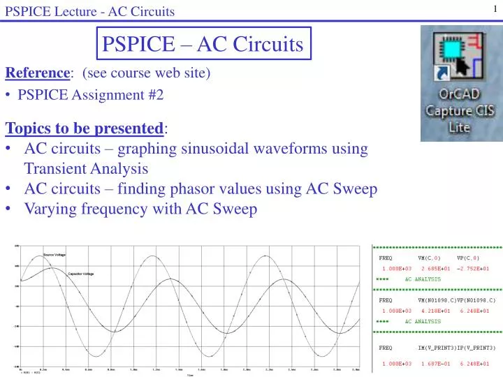
PSPICE Lecture - AC Circuits 1 PSPICE – AC Circuits • Reference: (see course web site) • PSPICE Assignment #2 • Topics to be presented: • AC circuits – graphing sinusoidal waveforms using Transient Analysis • AC circuits – finding phasor values using AC Sweep • Varying frequency with AC Sweep
PSPICE Lecture - AC Circuits 2 • AC Analysis in PSPICE • There are two common ways to analyze AC circuits in PSPICE: • Transient Analysis • Used for graphing sinusoidal waveforms • Time is varied, to time is on the x-axis of all graphs • Use the sources VSIN and ISIN • Angles referenced to sin( ), not cos( ) • AC Sweep • Used for calculating phasor voltages, phasor currents, etc (use the same starting and ending frequency for a single analysis) • Can also be used to vary frequency, so frequency (in Hz) is on the x-axis of all graphs • Use the sources VAC and IAC • Angles are relative. If you use angles referenced to sin( ), then angles are referenced to sin( ). If you use angles referenced to cos( ), then angles are referenced to cos( ).
PSPICE Lecture - AC Circuits 3 Example - Analyze the circuit below by hand. + VR - + VR - 250 250 + 50sin(2000t + 30o) V - + VC - + VC - 5030o V 1uF 1uF Solution: Phasor circuit: I + -
PSPICE Lecture - AC Circuits 4 Example (continued) Use PSPICE to graph v(t) and vC(t) for 3 periods. Solution: Since we want to graph the waveforms, used a transient analysis and use part VSIN for the source. 1) Create a New Project and draw the circuit in PSPICE. Since a transient analysis will be performed, use part VSIN for the voltage source. Add node labels as well. • Notes: Since v(t) = 50sin(2000t + 30), use the following values: • VOFF – This is the DC value. Use 0V. • VAMPL – This is the peak value of the sinusoid. Use 50V. • FREQ – This is the frequency in Hz. Use 1000Hz. • (continued on next slide)
PSPICE Lecture - AC Circuits 5 • Notes: (continued) • AC – This is the phasor voltage. We will use VAC instead for phasors. Delete this property. • PHASE – This is the phase angle in degrees. It does not show by default. Double-click on the part and select Edit Part. The Parts Editor window to the right should appear. Select the property named Phase. Select Display and change it to Name and Value. Close the Parts Editor. Enter 30 degrees for the phase. • The source below now has the correct values. • The units are not required, but are recommended.
PSPICE Lecture - AC Circuits 6 • Select PSPICE – New Simulation Profile • Analysis Type: Select Time Domain (Transient) • Run to time: Since T = 1/f = 1/1000 = 1ms, enter 3ms for 3 periods • Select OK.
PSPICE Lecture - AC Circuits 7 • Select PSPICE – Run • The graphing window should appear. • Select Trace – Add Trace • Select V(B) for the source voltage and V(C) for the capacitor voltage • Note that the voltages are a little choppy. This can be fixed by using more points for the analysis. By default PSPICE uses about 100 points so the time increment is about 3ms/100 = 30us. If we change this to 3us, PSPICE will use 1000 points instead of 100 points. See next slide.
PSPICE Lecture - AC Circuits 8 Blank value changed to 3us to use 3ms/3us = 1000 points for smoother graphs
PSPICE Lecture - AC Circuits 9 • Select Plot – Label – Text to add labels to each waveform • Select Window – Copy to Clipboardso that you can easily paste the graph into a Word document without the black background.
PSPICE Lecture - AC Circuits 10 • Example (continued) Use PSPICE to find the phasors • Solution: Since we want to find phasors, use an AC Sweep analysis and use part VAC for the source. • Create a New Project and draw the circuit in PSPICE. Since an AC Sweep will be performed, use part VAC for the voltage source. Add node labels as well. • Note that PSPICE only shows the values of two properties. Double-click on the part to open the parts editor. Select each property and change Display from Value Only to Name and Value. Also display Name and Value for the property named ACPHASE.
PSPICE Lecture - AC Circuits 11 • Notes: Since v(t) = 50sin(2000t + 30), use the following values: • ACMAG – This is the phasor magnitude. Use 50V. • ACPHASE – This is the phasor phase in degrees. Use 30degrees. • DC – This is the DC value. Use 0V or delete this property. • Units are not required, but are recommended.
PSPICE Lecture - AC Circuits 12 • Add voltage and current printers • An AC sweep analysis only calculates DC node voltages (typically all 0) by default. In order to find phasor voltages and currents, we must add printers. • Voltage Printers - must be placed in parallel with the desired component(s) • Current Printers – must be placed in series with the desired component(s) • Polarity – Note the (-) sign on each printer and rotate/flip if necessary for the correct voltage polarity or current direction. • For both printers set the following properties: • AC: Yes • MAG: Yes • PHASE: Yes Use part VPRINT2 for the voltage printer and part IPRINT for the current printer. Both are in the Special library.
PSPICE Lecture - AC Circuits 13 • Select PSPICE – New Simulation Profile • Analysis Type: Select AC Sweep/Noise • AC Sweep Type: Use the same Start Frequency and End Frequency (1000Hz in this case) for a single analysis. Even though the frequency isn’t actually being varied, a value must still be entered for Points/Decade • Select OK.
PSPICE Lecture - AC Circuits 14 • Select PSPICE – Run • View Results • The values from the voltage printers should now appear in the .OUT file. • Select PSPICE – View Output File • Note that the voltage printers express the voltages using node voltages • Add text to the Output file to clearly identify all results • A portion of the Output file is shown below: All results agree with the hand calculations!
PSPICE Lecture - AC Circuits 15 Example: Use PSPICE to graph total circuit impedance as frequency varies to show that |Z| is minimum at resonance. The circuit below is a series resonant circuit. As frequency increases XL becomes more positive and XCbecomes more negative. At the resonant frequency XL and XC cancel leaving a resistive circuit and minimum total impedance (equal to R).
PSPICE Lecture - AC Circuits 16 The resonant frequency is: Total impedance was calculated below as frequency varies from 100 to 10,000 Hz. Note that |Z| reaches a minimum at f = 500 Hz (close to the resonant frequency) We will now graph |Z| vs f in PSPICE to verify this result.
PSPICE Lecture - AC Circuits 17 • Create a new project and draw the circuit in PSPICE • Use part VAC for the source since an AC Sweep analysis will be performed. • Use any non-zero value for ACMAG and ACPHASE
PSPICE Lecture - AC Circuits 18 • Create a new Simulation Profile • Let frequency vary from 100Hz to 10000Hz • Frequency is typically shown on a log scale. • Select 50 points/decade (for a total of 100 points in this case)
PSPICE Lecture - AC Circuits 19 • Analyze the circuit- Select PSPICE – Run • Graph the results (PSPICE’s graphing window should open automatically) • Select Trace – Add Trace and enter V(A)/I(R1) for the total impedance • Use a cursor to mark the minimum point on the curve • Add text • The results are correct!