Download

1 / 65
650 likes | 659 Views
Continuum polarization of stars as a result of occultation by transiting exoplanets. N.G. Shchukina 1 , K. V. Frantseva 1 1 Main Astronomical Observatory, National Academy of Sciences, Ukraine J. Trujillo Bueno 2 2 Instituto de Astrofísica de Canarias, Spain.

E N D
Continuum polarization of stars as a result of occultation by transitingexoplanets • N.G. Shchukina1, K. V. Frantseva1 • 1Main Astronomical Observatory, National Academy of Sciences, Ukraine • J. Trujillo Bueno2 • 2Instituto de Astrofísica de Canarias, Spain Polarization as a tool to study the Solar System and beyond, Prague, 5-8 May 2014
Science objectives: To use polarimetry as a tool to detect and study ExoPlanets (EPs)
Techniques used for EPs discovery All exoplanets = 1026 Transiting Exoplanets = 402 http://exoplanetarchive.ipac.caltech.edu http:// var2.astro.cz/ETD Radial Velocity Transit Imaging Microlensing Eclipse timing variations; Pulsar timing variations; Orbital brightness variations; Astrometry
Stars with transiting exoplanetary systems Around 400 transiting EPs have been found to date (beginning of 2014)
The net linear polarization for a centrosymmetric star equals zero. Any asymmetry causes incomplete cancellation of stellar limb polarization and, as a result, the non-zero polarization. • Sources of asymmetry over the stellar disk: • spots • flattening by rotation • tidal perturbations • planetary atmospheres reflecting starlight • occultation effect, i.e. transit of EPs
The Stellar Continuum Polarization due to occultation effect
A planet observed with phase Ψand inclination i. μ = cos θis the angle between the normal to the star surface and the direction to the observer Transit of a 1 RJupiter ESP (solid circle) & 2 RJupiter ESP (dashed circle) in front a Sun-like star, for three different inclinations i
The observed normalized Stokes parameters q & u (in units of stellar flux) are: f and Pis the limb darkering and polarization, respectively − P0 Φ0 are polar coordinates of a system whose origin is Projected coordinates of the planet center in the plane of the sky are:
In order to estimate the continuum polarization caused by the occultation effect it is necessary to know the center-to-limb variation of the stellar continuum intensity f(the limb-darkering law) &the center-to-limb variation of the continuum polarization P in the stars under consideration.
First study Chandrasekhar S.(On the Radiative Equilibrium of a Stellar Atmosphere. X. 1946, ApJ, 103, 351)CASE:Polarized light in a pure Thomson scattering grey atmosphere (NO absorption opacity k = 0): P (μ) = 11.7% μ=0.0P (μ) = 0.3% μ=0.9
Recent studies The limb darkening is relatively well known for normal stars (Claret, A. 2000, A&A, 363, 1081) Stellar parameters: −5.0 ≤ log[M/H] ≤ +1, 2000K ≤ Teff ≤ 50000K and several surface gravities) Observational and theoretical studies of the continuum polarization are largely concentrated on the Sun.
Sun, 1D Fluri A.D., Stenflo J.O.1999, A&A, 341, pp. 902–911 One-dimensional (1D) radiative transfer modeling of the solar continuum polarization using plane-parallel, static atmosphere with homogeneous layers Sun, 3D HD Trujillo Bueno J., Shchukina N.G.2009, ApJ. 694, pp. 1364–1378 Three-dimensional (3D) radiative transfer modeling of the polarization of the Sun’s continuous spectrum using 3D hydrodynamical model
μ = 0.1 μ = 0.1 Wavelength variation of the polarization of the Sun’s continuous spectrum at μ = 0.1. The three blue dotted lines correspond to Stenflo’s (2005) semi-empirical determination, with the central curve showing the most likely representation. The solid and dashed lines show the Stokes Q/I in the 3D model (red lines) and in MACKKL model (black lines). Without spatial and/or temporal resolution U/I ≈ 0 and the only observable quantity is Q/I.
The results of such studies are usually adopted to calculate the continuum polarization resulting from occultation effects in given atmospheric models of several representantive late-type (mainly K,M,T dwarfs) stars. • 1D-case:Carciofi, A. C.; Magalhães, A.M., 2005, ApJ, 635,570 • 3D-case:Kostogryz N.M. et al. 2011,MNRAS, 415, 695 • Conclusion: • For the later spectral types, i.e. smaller stellar radii the polarization may be observable even for Earth-like planets (P > 10−5). • With large stellar radii the detection of the occultation polarization of Jupiter-like planets, down to Neptune-like planets, should be possible (P > 10−4).
Center-to limb polarization& limb darkering for a grid of F, G, K stars
A grid of Kurucz (1993) ATLAS9 atmospheres with overshooting Скорость Kurucz, R. L. 1993, CD-ROMs, ATLAS9 Stellar Atmospheres Programs and 2 kms−1 Grid (Cambridge: Smithsonian Astrophys.Obs.) Total number: 150 models[Me/H] = -0.5 0.0 0.5Teff = 4600 4800 5000 5200 5400 5600 5800 6000 6200 6400log g = 3.0 3.4 4.0 4.4 4.8
Typical samples of stars used in this study Sun TrES-3WASP-4CoRoT-2 HD189733 6400 4600 Teff 5777 572254935204 4954 6400 4600 Log g 4.44 4.594.504.524.59 4.00 3.00 [Me/H] 0.0 −0.18−0.10−0.15−0.18 0.0 −0.5 Sp.class G2V G4V K2V K0VK1V F K
The physical mechanisms • Scattering: • The polarization of the F, G, K star´s continuous radiation is caused by: • Thomson scattering at free electrons • Rayleigh scattering from the ground level of neutral hydrogen • Rayleigh scattering by H2 molecules is a dominant source of opacity at shorter wavelengths in M type stars. (Tsuji T., 1966, Publ. Astron. Spoc. Japan, 18,127-173 ) • Continuum pure absorption : • bound–free and free–free transitions in H−, • bound–free and free–free transitions in hydrogen, • bound–free transitions in C, Si, Fe, Mg, Al • UV haze (λ≤ 4500 Å) (Bruls, J. H. M. J., Rutten, R. J., & Shchukina, N. G. 1992, A&A, 265, 237) • See details in: • Trujillo Bueno J. & Shchukina N. Three-dimensional radiative transfer modeling of the polarization of the sun’s continuous spectrum,ApJ, 2009, 694, 1364
Numerical solution is based on the iterative methods developed by Trujillo Bueno J. & Manso Sainz R. (1999, ApJ, 1999, 516,436): Since the atmosphere is one-dimensional, the radiation field has rotational symmetry with respect to the vertical to the stellar atmosphere and the only nonvanishing Stokes parameters are I and Q. We calculate the center-to limb polarization P (μ) = Q (μ) /I(μ) & limb darkering f(μ) =I (μ) /I(μ=1)
High sensitivity of the continuum limb darkering I(μ=0.1)/I(μ=1) to wavelength The variation with wavelength of the continuum intensity for μ=0.1, normalized to the disk center value.
High sensitivity of the continuum polarization Q(μ)/I(μ) to wavelength Wavelength variation of the continuum polarization Q/I for representative stars. μ=0.1
High sensitivity of Q/I to logg & Teff Variation of the continuum polarization Q/I with effective temperatureTeff, gravitylog g&metallicity [Me/H]at the stellar limbμ=0.1. λ=3700 Å
The limb-darkering functions for F,G, K stars are well described by by the polynomial approximation of the 4th order: I(μ)/I(μ=1) = D0 + D1∙x + D2∙x2 + D3∙x3 + D4∙x4 x = √μ Di = f(λ, Teff, logg, [Me/H])
The center-limb variation of the continuum polarization Q/I for F, G, K is well described by by the polynomial approximation of the 6th order: Q(μ)/I(μ) = Q0 + Q1∙x + Q2∙x2 + Q3∙x3 + Q4∙x4 + Q5∙x5 + Q6∙x6 Qi = f(λ, Teff, logg, [Me/H]) Use of of Chandrasekhar´s approximation for description of the continuum polarization Q/I in F, G, K stars (see Kostogryz N.M. et al. 2011) is erroneous.
Modeling the occultation continuum polarization for a grid of F, G, K stars
We used a Monte Carlo integrator for solving eqs Since the atmosphere is one-dimensional, the radiation field has rotational symmetry with respect to the vertical to the stellar atmosphere and the only nonvanishing Stokes parameters are I(μ) and Q(μ).
Hot Jupiters R (star) = R (Sun) R (planet) = R(Jupiter) A = 0.04 AU Period = 2.93 days Inclination = 87o Mass (star) >> M (planet)
HD189733: P ≈ 10-5 Sun: P ≈ 10-6 Modelled curves for two stars. From top to the bottom: normalized flux at 4200 Å; normalized Stokes q; Stokes u parametes; occultation polarization.
The Johnson-Cousins B filter Stars with transiting exoplanetary systems plotted over max value Pmax of the occultation polarization at λ=4200 Å. Pmax = f (Teff, log g)
λ=4600 Ǻ Stars with transiting exoplanetary systems plotted over max value of the occultation polarization at λ=4600 Å. The black line indicates the best polarization sensitivity for current broadband polarimeters (P=1·10-6).
The Johnson-Cousins V filter Stars with transiting exoplanetary systems plotted over max value of the occultation polarization at λ=5300 Å. The black line indicates the best polarization sensitivity for current broadband polarimeters (P=1·10-6).
Thus, the occultation polarization signal is small. Is it possible the high accuracy for EPs polarimetric detection and study ? A sensitivity of highly accurate polarimetry for EPs detection can be better than 10−6 Kemp et al. , 1987, Nature, 326, 270 J. C. Kemp, 1988, private communication Hough et al., 2006, PASP,118, 1302
Summary • Center-to limb polarization Q/I, limb darkering f and occultation polarization for a grid of F, G, K stars are available in electronic format both for the monochromatic “observations” (3000 Å to 8000 Å) & for the Johnson-Cousins UX, B, V, R, I filters. • The results were obtained for the following stellar parameters: metallicity ranging from −0.5 up to +0.5, gravity varying between 3.0 and 4.8 and effective temperatures between 4600 K−6400 K. • Occultation polarization signal produced during hot Jupiters transits over F, G, K stars can be measured using filters with bandpass at wavelengths less than 4600 Ǻ.
Thank you for your attention
Sources of the stellar continuum polarization • The Stellar Polarization due to Light Transmission Through the Interstellar Dust Medium • The Intrinsic Stellar Continuum Polarization
The observed polarization of any distant star located • near the Galactic plane may have a nonzero interstellar component: • Interstellar linear polarization is caused by the linear dichroism of the interstellar medium due to the presence of non-spherical aligned grains. • Dust grains must have sizes close to the wavelength of the incident radiation and specific magnetic properties to efficiently interact with the interstellar magnetic field. • The direction of alignment must not coincide with the line of sight and there must be no cancellation of polarization during the propagation of radiation through the interstellar medium. • Grains:infinite cylinders, silicate core–ice mantle, silicate core–organic, silicate spheroids with graphite inclusions, dust aggregates • See details in: • N.V. Voshchinnikov. Interstellar extinction and interstellar polarization: old and new models, JQSRT, 2012, Vol. 113, Issue 18, p. 2334-2350
Interstellar polarization was first discovered inthe 1940s byDombrovsii V.A.(On the polarization of radiation of early-type stars. Doklady Akad Nauk Armenia. 1949, 10, pp.199–203). This phenomenon was observedindependently byHiltner & Hall (Hiltner W.A. Polarization of light from distant stars by interstellar medium. 1949, Science; 109: pp.165–165; 1949, ApJ, 109, 471 Hall J.S. Observations of the polarized light from stars, 1949; Science, 109:166–167). Such a polarization is found only in distant stars, and there is a correlation between the degree of polarization P, the modulus of the distance m−M and color excess E (Sobolev, V.V. Course of Theoretical Astrophysics,1967, Nauka, Moscow). Observations show that the degree of polarization is small (less than a percent or a few percent), but in some cases reaches 10%.
The interstellar polarization of stars in the local ionized bubble within ~100 pc of the Sun is very small: typically P ~ 10−5 – 10−6 Hough, J. H.; Lucas, P. W.; Bailey, J. A.; Tamura, M.; Hirst, E.; Harrison, D.; Bartholomew-Biggs, M. PlanetPol: A Very High Sensitivity Polarimeter 2006, PASP, 118, Issue 847, pp. 1302-1318
Stars with transiting exoplanetary systems • The net linear polarization for a centrosymmetric star equals zero. Any asymmetry causes incomplete cancellation of stellar limb polarization and, as a result, the non-zero polarization. • Sources of asymmetry over the stellar disk: • spots • flattening by rotation • tidal perturbations • planetary atmospheres reflecting starlight • occultation effect, i.e. transit of ESPs
Chandrasekhar S.(On the Radiative Equilibrium of a Stellar Atmosphere. X. 1946, ApJ, 103, 351)CASE:Polarized light in a pure Thomson scattering grey atmosphere (NO absorption opacity k = 0): P (μ) = 11.7% μ=0.0P (μ) = 0.3% μ=0.9 Code A.D.(Radiative equilibrium in an atmosphere in which pure scattering and pure absorption both play a role,1950, ApJ. 112, 22)CASE:Polarized light in a pure Thomson scattering (σ is wavelength independent) grey atmosphere (WITH absorption opacity k ≠ 0): hot stars, Te ~10000, 20000 K free parameterλ=k/(σ+k)P max= 0.5% λ=0.5 μ=0.9P max= 11.3% λ=0.0 μ=0.0
Spectropolarimetry of supernovae (Dessart, L.; Hillier, D. J. 2011, MNRAS, 415, 3497) • Spectropolarimetry of accretion disk around a supermassive black hole: Lyman continuum (Shields, G. A.; Wobus, L.; Husfeld, D. 1998, ApJ, 496, 743) Polarization is about a few percent ?
Sun, 1D Fluri A.D., Stenflo J.O.1999, A&A, 341, pp. 902–911 A plane-parallel, static atmosphere with homogeneous layers:9 1D Solar model atmospheres.Stokes Q represents linear polarization with respect to the direction parallel to the nearest solar limb, so Stokes U = V = 0.scattering coefficientσc: Thomson scattering at free electronsRayleigh scattering atneutral hydrogen.Absorption coefficient kc: mainly due to H−.Continuum from 4000 Å to 8000 Å P(μ)=P1(1 −μ2)/(1+kμ), kis a measure of the width of the polarization profile (i.e., the larger the k, the faster the polarization drops from the value at the limb).
Sun, 3D HD Trujillo Bueno J., Shchukina N.G.Three-dimensional radiative transfer modeling of the polarization of the Sun’s continuous spectrum,2009, ApJ. 694, pp. 1364–1378 Q/I ≈ 3/2√2 (1 −μ2) ∙σc/(σc + kc)∙α∙J20/J00 σc/(σc + kc) is the effective polarizability J20/J00 anisotropy of the continuum radiation, μ=cos Θ LOS with Θbeing the polar angle, α = f(λ) ≈ 2 - 4
The height variation of the mean continuum intensity J00 and anisotropy J20/J00 at λ=4600 Å for all the horizontal grid points of the 3D model. The blue curves correspond to the upflowing regions of the 3D model and the red ones correspond to the downflowing ones.
The behavior of the continuum polarization calculated in the 3D model. Each curve gives the center-limb variation of the continuum polarization for the indicated wavelengths.
3D RT modeling takes into account not only the anisotropy of the solar continuum radiation but also the symmetry-breaking effects caused by the horizontal atmospheric inhomogeneities produced by the solar surface convection. Such symmetry-breaking effects produce observable signatures in Q/I and U/I, even at the very center of the solar disk. λ= 4600 Å
Variation of the continuum polarization Q/I with effective temperature Teff, gravity log g and metallicity [Me/H] at the stellar limb μ=0.1. λ=7000 Å