Download
1 / 37
710 likes | 1.41k Views
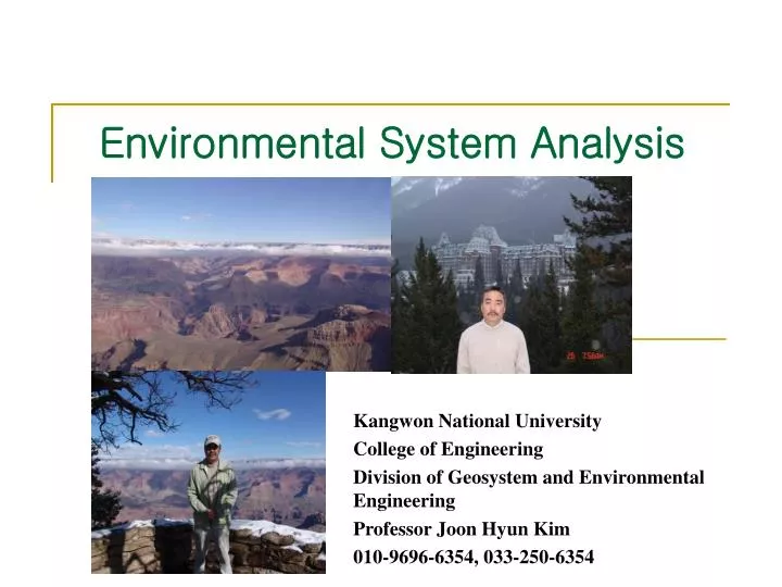
Environmental System Analysis. Kangwon National University College of Engineering Division of Geosystem and Environmental Engineering Professor Joon Hyun Kim 010-9696-6354, 033-250-6354. Class Contents and Schedule. Environmental Modeling.

E N D
Environmental System Analysis Kangwon National University College of Engineering Division of Geosystem and Environmental Engineering Professor Joon Hyun Kim 010-9696-6354, 033-250-6354
Environmental Modeling Fate and Transport of Pollutants in Water, Air, and Soil -JERALD L. SCHNOOR
1. INTRODUCTION If we are going to live so intimately with these chemicals, eating and drinking them into the very marrow of our bones, we had better know something about their nature and power -Rachel Carson, Silent Spring
1.1 SCOPE OF ENVIRONMENTAL MODELING Why should we build mathematical models of environmental pollutants? 1) To gain a better understanding of the fate and transport of chemicals by quantifying their reactions, speciation, and movement for the prediction of fate, transport, and persistence of chemicals in the environment. • Classic models address conventional pollutants, eutrophication, toxic organic chemicals, and metals in surface waters and groundwater. • Recently, mathematical models have become more sophisticated in terms of their chemistry. This book seeks to solidify the bond between water quality modeling and aquatic chemistry. Chemical speciation models are coupled with kinetic transport models for determining fate and chemical speciation.
2) To determine chemical exposure concentrations to aquatic organisms and/or humans in the past, present, or future. • It pertains to assessing the effects of chemical pollutants. New water quality criteria are promulgated to account for acute and chronic effects levels using frequency and duration of exposure. • These criteria result in water quality standards that are enforceable by law and require the application of mathematical models for waste load allocations, risk assessments, or environmental impact assessments. • Toxic chemicals-ammonia, arsenic, cadmium, chlorine, chromium, copper, cyanide, lead, and mercury-have been regulated. The criteria specify an acute threshold concentration and a chronic-no-effect concentration for each toxicant as well as tolerable durations and frequencies. • New criteria recognize that toxic effects are a function both of the magnitude of a pollutant concentration and of the organism exposure time to that concentration : (1) the 4-day average concentration of the toxicant does not exceed the recommended chronic criterion more than once every three years on the average and (2) the 1-hour average concentration does not exceed the recommended acute criterion more than once every three years on the average.
3) To predict future conditions under various loading scenarios or management action alternatives. • Waste load allocations and exposure models for risk assessment fall into this category. • Regardless how much monitoring data are available, it will always be desirable to have an estimate of chemical concentrations under different conditions, results for a future waste loading scenario, a predicted "hindcast" or reconstructed history, or estimates at an alternate site where field data do not exist. • For all these reasons we need chemical fate and transport models, and we need models that are increasingly sophisticated in their chemistry, as we move toward site-specific water quality standards and chemical speciation considerations in ecotoxicology. • To model aquatic chemical systems, we begin with a simple mass balance based on the principle of continuity: matter is neither created nor destroyed in macroscopic chemical, physical, and biological interactions.
1.2 MASS BALANCES • Water quality may be defined as "something inherent or distinctive about water." These distinctive characteristics can be chemical, physical, or biological parameters. • Mass balance serves for determining the fate of water quality parameters in natural waters and to assess degree of pollution expected under various conditions • The fate of chemicals in the aquatic environment is determined by • their reactivity • the rate of their physical transport through the environment • Mathematical models are simply useful accounting procedures for the calculation of these processes • To the extent that we can accurately predict the chemical, biological, and physical reactions and transport of chemical substances, we can "model" their fate and persistence and the inevitable exposure to aquatic organisms • Key elements in a mass balance (see Fig.1.1): (i) A clearly defined control volume. (ii) A knowledge of inputs and outputs that cross the boundary of the control volume. (iii) A knowledge of the transport characteristics within the control volume and across its boundaries. (iv) A knowledge of the reaction kinetics within the control volume.
A control volume: • can be as small as an infinitesimal thin slice of water in a swiftly flowing stream or as large as the entire body of oceans on the planet earth. • The important point: the boundaries are clearly defined with respect to their location (element i) so that the volume is known and mass fluxes across the boundaries can be determined (element ii). • Transport in adjacent or surrounding control volumes may contribute mass to the control volume, so transport across the boundaries of the control volume must be known or estimated (element iii). • A knowledge of the chemical, biological, and physical reactions that the substance can undergo within the control volume (element iv) is needed. Figure 1.1 Generalized approach for mass balance models utilizing the control-volume concept and transport across boundaries.
Mass balance: Classification of substances relative to their reactions in water
Mass Balance of Water (Water Balance, Water Budget) • If the system is nearly isothermal, then the mass of storage is accounted for by the volume of inflows and outflows. • inflows: the volumetric inputs of tributaries and overland flow • outflows: all discharges from the water body • direct precipitation: water that falls directly on the surface • evaporation: volume of water that leaves the surface of the water body to the atmosphere. • In case of inputs/outputs of groundwater, the piezometric surface of the groundwater adjacent to the water body must be measured . Q = flow rate m3d-1 I = precipitation rate md-1 A = surface area of water body, m2 E = evaporation rate md-1 ∆t = time increment, days ∆V = change in storage volume, m3
Figure 1.2 Schematic of a lake with inflows and outflows for computation of a water budget
Example 1.1 Mass Balance of Water (Volume) in a Lake Calculate the volume of a lake over time during a drought if the sum of all inputs is 100 m3s-1 and the outflows are 110 m3s-1 and increasing 1 m3s-1 every day due to evaporation and water demand. Initial volume of the lake is 1 × 10⁹ m3. See Figure 1.3. (Note : Convert all units from seconds to days.) Solution:
Figure 1.3 Plot of volume versus time for hypothetical lake during a drought period
Example 1.2 Algebraic Mass Balance on Toxic Chemical in a Lake Calculate the steady-state concentration of a toxic chemical in a lake under the following conditions. Assume steady state (dC/dt = 0) and constant volume (Qin = Qout) and a degradation rate of 50 kg d-1 for the conditions such as : Cin=100μgL-1, Qin=Qout=10m3s-1, -Rxn=50kgd-1 Solution: Write the mass balance equation for the lake as a control volume Accumulation = Inputs - Outflows ± Rxns , Accumulation = 0 at steady state Outflows = Inputs - Rxn (degradation)
1.3 MODEL CALIBRATION AND VERIFICATION O To perform mathematical modeling, four ingredients are necessary: 1) field data on chemical concentrations and mass discharge inputs 2) a mathematical model formulation 3) rate constants and equilibrium coefficients for the mathematical model 4) some performance criteria with which to judge the model O If the model is to be used for regulatory purposes, there should be enough field data to be confident of model results (two sets of field measurements, one for model calibration and one for verification under somewhat different circumstances (a different year of field measurements or an alternate site) O Model calibration involves a comparison between simulation results and field measurements. Model coefficients and rate constants should be chosen initially from literature or laboratory studies. O If errors are within an acceptable tolerance level, the model is considered calibrated. If errors are not acceptable, rate constants and coefficients must be systematically varied (tuning the model) to obtain an acceptable simulation. The parameters should not be "tuned" outside the range of experimentally determined values reported in the literature. O After you run the model, a statistical comparison is made between model results for the state variables (chemical concentrations) and field measurements. The model is calibrated.
Definition of Terminologies • Mathematical model-a quantitative formulation of chemical, physical, and biological processes that simulates the system. • State variable-the dependent variable that is being modeled (in this context, usually a chemical concentration). • Model parameters-coefficients in the model that are used to formulate the mass balance equation (e.g., rate constants, equilibrium constants, stoichiometric ratios). • Model inputs-forcing functions or constants required to run the model (e.g., flowrate, input chemical concentrations, temperature, sunlight). • Calibration-a statistically acceptable comparison between model results and field measurements; adjustment or "tuning" of model parameters is allowed within the range of experimentally determined values reported in the literature. • Verification-a statistically acceptable comparison between model results and a second (independent) set of field data for another year or at an alternate site; model parameters are fixed and no further adjustment is allowed after the calibration step.
Simulation-use of the model with any input data set (even hypothetical input) and not requiring calibration or verification with field data. • Validation-scientific acceptance that (1) the model includes all major and salient processes, (2) the processes are formulated correctly, and (3) the model suitably describes observed phenomena for the use intended. • Robustness-utility of the model established after repeated applications under different circumstances and at different sites. • Post audit-a comparison of model predictions to future field measurements at that time. • Sensitivity analysis-determination of the effect of a small change in model parameters on the results (state variable), either by numerical simulation or mathematical techniques. • Uncertainty analysis-determination of the uncertainty (standard deviation) of the state variable expected value (mean) due to uncertainty in model parameters, inputs, or initial state via stochastic modeling techniques.
Statistical Analysis • Statistical "goodness of fit" criteria using chi-square or Kolmogorov-Smirnov tests (tests of the sampling distribution of the variance). • Paired t-tests of model results and field observations at the same time (a test of the means). • Linear regression of paired data for model predictions and field observations at the same time. • A comparison of model results to field observations and their standard deviation (or geometric deviation, if appropriate). • Parameter estimation techniques such as nonlinear curve-fitting regressions (weighted or unweighted) or Kalman filters to determine model parameters in an optimal fashion.
Model Verification • To verify the model, a statistical comparison between simulation results and a second set of field data is required. • Coefficients and rate constants cannot be changed from the model calibration. • Acceptance of a model calibration of verification does not necessarily imply that the model, itself, is validated. It is possible that the model works well under one set of circumstances but poorly under another. As the model is applied to different situations at various locations, we gain confidence in the model and its robustness. The process when the model is considered validated is gradual. • Further testing its formulation and validity. • Post audits of model results are an important test of the usefulness of the model (they are performed after model predictions have been made as data become available in the future). Very few post audits have been reported in the literature. More are needed.
Example 1.3 Calibration and Criteria Testing of a DO Model for a Hypothetical Stream A water discharge with biochemical oxygen demand (BOD) at km 0.0 causes a depletion in dissolved oxygen in a stream (D.O. sag curve). Model calibration results are tabulated below (D.O. model) together with field measurements (D.O. field) expressed in concentration units, mg L-1. See Figure 1.4. Determine if the model calibration is acceptable according to the following statistical criteria: a. Chi-square goodness of fit at a 0.10 significance level (a 90% confidence level). b. Paired t-test (difference between the mean and zero) at significance level c. Linear least-squares regression of model results (D.O. model on x-axis) versus observed data (D.O. field data on y-axis) with r2 > 0.8.
Figure 1.4 Dissolved oxygen model calibration and comparison to field measurements.
Chi-Square Fitness Test where the observed values are the D.O. field data, and the expected values are the D.O. model results. α is the confidence level and χ02 is the chi-square distribution value for n-1 degrees of freedom. χ02=4.17 for n = 10 and α= 0.9. The value for χ02 = 4.17 was determined from a statistical table for the chi-square distribution with 9 degrees of freedom (n-1) and P = 0.10. The table below shows that 0.1254≤4.17. Therefore the model passes the goodness of fit test at a 0.10 significance level.
Paired T-Test di - difference between values in data pairi. The acceptance criterion for the t-test for n-1 degrees of freedom is In D.O model the value 1.833 wart determined from a table t-values with 9 degrees of freedom and P = 0.10. The above shows The test statistic can be calculated The model results are found to be indistinguishable from the field data at a significance level of 0.10 from the paired t-test because 0.3699≤1.833.
Linear Least Square Regression Analysis Test Perfect model predictions would yield • The D.O. model meets the linear regression criteria of r2>0.8. • It would have been better to have more observations (field data) to test the model. • All three models become more powerful (in the statistical sense) as n→30 data points.
1.4 ENVIRONMENTAL MODELING AND ECOTOXICOLOGY • Environmental modeling is the attempt to understand better the fate of chemicals in our environment and the role of humans in those chemical cycles. • We are impacting larger and larger domains: oceans, not just coastal waters; the stratosphere, not just urban air; deep groundwater aquifers, not just surface waters. • In industrialized nations, the anthropogenic energy flow per unit area exceeds photosynthesis by a factor of about 10. • Despite intensive research, we only partially understand how chemical pollutants move between atmosphere, land, and water and what transformations they undergo during transport. . • Some 1000-1500 new chemicals are manufactured each year with perhaps 60,000 chemicals in daily use (mostly organic chemicals). Table 1.2: list of some priority pollutants with their various transformation reactions. • We have made progress during the past ten years at predicting rates of reaction and partitioning. However, less progress has been made on predicting biotransformation. • Heavy metal pollutants are pervasive and, perhaps, are a greater problem than organic chemicals based on their persistence . • Generally human activities cause elevated concentrations of metals (Figure 1.5).
Table 1.2 Priority Organic Chemicals and Their Reactions Significant reactions for selected priority pollutant organic chemicals in natural waters
Figure 1.5 Periodic table and average freshwater concentration
Phosphate, nitrate, and ammonium are nonpoint source problems from agricultural runoff that continue to cause the eutrophication of surface waters, oxygen depletion of sediments, habitat alteration, and ecological changes in the structure and function of the ecosystem that are often difficult to detect, quantify, and prevent . • The ability of a trace element to pose an environmental hazard depends not only on its enrichment in the atmosphere or hydrosphere but also on its chemical speciation (form of occurrence) and the details of its biochemical cycling. Bioavailability and toxicity depend strongly on the chemical species. For algae and lower organisms, the free metal aquo ions often determine the physiological and ecological response . • At present the open ocean and many lakes are more affected by pollution impacts through tropospheric transport than through riverine transport. Elements are termed atmophile when their mass transport to the sea is greater from the atmosphere than from transport by streams. This is the case for Cd, Hg, As, Se, Cu, Zn, Sn, and Pb. Atmophile elements are either volatile, or their oxides or other compounds have low boiling points. • The elements Hg, As, Se, Sn, and perhaps Pb can also become methylated and are released in gaseous form into the atmosphere. The elements Al, Ti, Mn, Co, Cr, V and Ni are termed lithophiles because their mass transport to the ocean occurs primarily by streams.
Soft Lewis acids, metals such as Cu+, Ag+, Cd2+, Zn2+, Hg2+, and Pb2+, and the transition metal cations (Mn2+, Fe2+, Ni2+, Cu2+) are of environmental concern, both from a point of view of anthropogenic emissions as well as hazard to ecosystems and human health (chemical reactivity with biomolecules) . Considering the schematic reaction, Igneous rock + Volatile substances = Air + Seawater + Sediments • Volatiles such as H2O, CO2, HCl, and SO2, that have been emitted from volcanos after being leaked from the interior of the earth, have reacted in a gigantic acid-base reaction with the bases of the rocks. On the global average, the environment with regard to a proton and electron balance is in a stationary situation, which reflects the present-day atmosphere (20.9% O2, 0.03% CO2, 79.1% N2), an ocean pH of~8, and a redox potential corresponding to a partial pressure of O2 equal to 0.21 atm. • The weathering cycle is affected markedly at least locally and regionally by our civilization. In local environments H+ and e- balances may become upset and significant variations in pH occur. • The reactions of the oxidation of C, S, and N exceed reduction reactions in these elemental cycles. A net production of hydrogen ions (acids) in atmospheric precipitation is a necessary consequence. Many mere potential atmospheric pollutants (photooxidants, polycyclic aromatic hydrocarbons smog particles, etc.) are formed under the influence of photochemically induced interactions with OH radicals, H2O2, ozone, and hydrocarbons with fossil fuel combustion products. • The atmosphere has become an important conveyor belt for many potential aquatic pollutants. Many persistent pollutants are present in a vapor phase during transport from land to fresh water and from continent to ocean. These substances include many pesticides, such as DDT, more volatile metals (Hg), metalloids (As, Se), or their compounds. At present the open ocean is probably more affected by metal pollution inputs through tropospheric transport than through rival transport (Pb).
Figure 1.6 Comparison of global reservoirs The reservoirs of atmosphere, surface fresh waters. and living biomass are significantly smaller than the reservoirs of sediment and marine waters. The total groundwater reservoir may be twice that of fresh water. However, groundwater is much less accessible.
In Figure 1.6 the sizes of the various reservoirs, measured in number of molecules or atoms, are compared. The mean residence time of the molecules in these reservoirs is also indicated. The smaller the relative reservoir size and residence time, the more sensitive the reservoir toward perturbation. • Obviously, the atmosphere, living biomass (mostly forests), and ground and surface fresh waters are most sensitive to perturbation. The anthropogenic exploitation of the larger sedimentary organic carbon reservoir (fossil fuels and by-products of their combustion such as oxides and heavy metals and the synthetic chemicals derived from organic carbon) can above all affect the small reservoirs. • The living biomass (Figure 1.6) is a relatively small reservoir and thus subject to human interference; each species forming the biosphere requires specific environmental conditions far sustenance and survival. • Transport of pollutants from air to water and from land to water have become increasingly important pathways for the occurrence of water pollution (Figure 1.7). Degradation of groundwater from soil pollution is a major environmental problem (c.g., infiltration of pesticides from agricultural applications or leachate from hazardous waste landfills). Also, impacts of acid deposition on surface waters and oxidants on forests and soils illustrate the importance of transport through the airwater interface. We need to know about the aquatic chemistry of these pollutants to estimate their speciation and fete in the environment, and we need to know how to construct and solve mathematical models (mass balance equations) to calculate simultaneously their transport and transformations.
Figure 1.7 Path of a pollutant through the environment The distribution of a pollutant in the environment is dependent on its specific properties. Of particular ecological relevance is fat solubility or lipophilicity, as lipophilic substances accumulate in organisms and the food chain. Biodegradation and chemical or photochemical decomposition decrease residence time and residual concentrations.
Figure 1.8 Transfer and transformation of pollutants in aquatic ecosystems A substance introduced into the system becomes dispersed diluted. It can become eliminated firm the water by adsorption on particles or by volatilization. It may also be transformed chemically or biologically.
Figure 1.8: synopsis of the perspectives of aquatic ecotoxicology. Let us follow the various steps from the source to the potential ecological effects of a pollutant released into an aquatic ecosystem. The emission is measured as a flow or Input load (capacity factor; mass per unit time or mass per unit time and volume or area). The resulting concentration is a consequence of the dilution, transport, and transformation of this chemical. At any point, the water condition is characterized by the interacting physical, chemical, and biological factors. • The ecological damage of a substance depends on its interaction with organisms or with communities of organisms (Figure 1.8). The intensity of this interaction depends on the specific structure and activity of the substance under consideration, but other factors such as temperature, turbulence, and the presence of other substances are also important. • An understanding of the interaction of chemical compounds in the natural system hinges on the recognition of the compositional complexity of the environment requires analytical methodology: ability to predict individual components selectively, measure them, forecast their fate. Table 1.3 lists water quality criteria toxicity thresholds, carcinogenicity, and maximum contaminant levels (M.C.L.) for many toxic chemicals discharged to natural waters. • Water quality criteria are the best scientific information from toxicological studies of the maximum concentration allowable that will not cause an observable biological effect. As ecotoxicology becomes more sophisticated as a science, the list of chemicals will grow and species specific criteria will be promulgated under various environmental conditions.