Download
1 / 29
310 likes | 509 Views
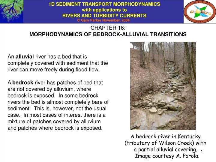
CHAPTER 16: MORPHODYNAMICS OF BEDROCK-ALLUVIAL TRANSITIONS. An alluvial river has a bed that is completely covered with sediment that the river can move freely during flood flow.

E N D
CHAPTER 16: MORPHODYNAMICS OF BEDROCK-ALLUVIAL TRANSITIONS An alluvial river has a bed that is completely covered with sediment that the river can move freely during flood flow. A bedrock river has patches of bed that are not covered by alluvium, where bedrock is exposed. In some bedrock rivers the bed is almost completely bare of sediment. This is, however, not the usual case. In most cases of interest there is a mixture of patches covered by alluvium and patches where bedrock is exposed. A bedrock river in Kentucky (tributary of Wilson Creek) with a partial alluvial covering. Image courtesy A. Parola.
THE CONCEPT OF TRANSPORT CAPACITY Equilibrium bedrock streams transport alluvium under below-capacity conditions, whereas alluvial streams transport sediment under at-capacity conditions. These concepts can be explained as follows. If the sediment supply of an alluvial river is increased, the bed can be expected to aggrade toward a new, steeper slope capable of carrying the extra sediment. A bedrock stream, on the other hand, may experience no aggradation when sediment supply is increased. Instead, the stream responds by reducing the fraction of the bed covered by bedrock and increasing the fraction covered by alluvium. Only when the bed is completely covered with alluvium can the river respond to increased sediment supply by aggrading. Big Box Creek, USA, a bedrock river with a stepped profile. Image courtesy E. Wohl.
QUANTIFICATION OF TRANSPORT CAPACITY The concept of a mobile-bed equilibrium state was outlined in Chapter 14. In the case of the Chezy resistance relation and the sample sediment transport relation introduced in that chapter, the governing equations of this equilibrium state take the following forms: Now let grain size D, sediment submerged specific gravity R, resistance coefficient Cf, critical Shields number c* and the parameters g, t and nt be given. The relations specify two equations in the following four parameters: depth H, bed slope S, water discharge per unit width qw and volume total bed material sediment discharge per unit width qt. Consider a stream with given values of water discharge per unit width qw and bed slope S. The capacity transport qt is that computed from the above equation.
BELOW-CAPACITY CONDITIONS Now suppose that for given values of qw and S, the actual sediment supply qts is less that the value qt associated with mobile-bed equilibrium, i.e. An alluvial stream would degrade to a lower slope S that would allow the above equation to be satisfied with qts. A bedrock stream, however, cannot degrade. So in the event that for given values of qw and S the sediment supply rate qts is less than the equilibrium mobile-bed value qt, the river responds by exposing bedrock on its bed instead of degrading. As qts is further reduced the river responds by increasing the fraction of the bed over which bedrock is exposed (Sklar and Dietrich, 1998). The river so adjusts itself to transport sediment at the rate qts which is below its capacity qt for the given values of qw and S. This allows a below-capacity equilibrium. In the event that the actual sediment supply qts is greater than the capacity transport rate qt at the given slope S , the river will aggrade to a new, higher slope in consonance with qts that satisfies the above equation. There is no above-capacity equilibrium.
A SAMPLE CALCULATION The following values are assumed in the sediment transport relation below: t = 3.97, nt = 1.5, c* = 0.0495 (Wong and Parker, submitted, modification of Meyer-Peter and Müller), R = 1.65, g = 9.81 m2/s and Cf = 0.01. Consider a river with D = 20 mm, flood Qw = 90 m3/s and width B = 30 m. The flood value of qw = Qw/B = 3 m2/s. For any slope S, then, the capacity value of qt can be computed from the above relation. Assume that a bedrock river is just barely completely covered with alluvium at the slope S. How will the river respond if sediment supply qts is reduced or increased? The following two slides illustrate that the river will aggrade to a new mobile-bed equilibrium when qts > qt. When qts < qt, the river cannot degrade due to the presence of bedrock, and instead reaches a below-capacity equilibrium with exposed bedrock.
ILLUSTRATION OF BELOW-CAPACITY TRANSPORT OF 7 MM GRAVEL OVER A BEDROCK BED The video clip is from the Ph.D. research of Phairot Chatanantavet. rte-bookbelowcaptrans.mpg: to run without relinking, download to same folder as PowerPoint presentations.
BEDROCK-ALLUVIAL TRANSITIONS: THE “FALL LINE” The southeastern coastal plain of the United States is characterized by a feature called the “Fall Line.” Upstream (westward) of this line the streams are in bedrock. Downstream (eastward) of this line they are in alluvium. It is of interest to speculate how the position of the fall line might respond to changing sea level. Image of the southeastern coastal plain of the United States from NASA https://zulu.ssc.nasa.gov/mrsid/mrsid.pl
EQUILIBRIUM STATE WITH BEDROCK-ALLUVIAL TRANSITION A bedrock channel has constant slope Sb and carries flood discharge per unit width qw. Sediment with size D is fed in at the upstream end at rate qts. The at-capacity slope S consonant with qst, qw and D (as computed, for example, from the transport relation of Slide 5) is less than Sb. Base level is maintained at some elevation at the downstream end; this level is higher than the elevation of the bedrock basement there. An equilibrium bedrock-alluvial transition must occur. To find it, draw a straight line with slope S and intercept at the point of base level maintenance, and extend it upstream until it intersects the bedrock profile.
DYNAMICS OF THE MIGRATION OF BEDROCK-ALLUVIAL TRANSITIONS Bedrock-alluvial transitions can migrate upstream or downstream due to the effects of e.g. changing sediment supply from upstream or changing base level downstream. The figure below shows a case where the alluvial region is (for whatever reason) aggrading, resulting in an upstream migration of the bedrock-alluvial transition.
CONTINUITY CONDITION AT THE BEDROCK-ALLUVIAL TRANSITION The elevation profile of the bedrock basement is denoted as base(x); it is assumed to be unchanging in time. The elevation profile of the alluvial zone is denoted as (x, t); it can change in time due to aggradation or degradation. The position of the bedrock-alluvial transition is denoted as x = sba(t). It is a function of time because the position of the transition can change in time. In order for the bedrock channel to join continuously with the alluvial channel, the following condition must hold: or Now take the derivative with respect to time of both sides of the equation. For example, where S = -/x denotes the alluvial bed slope and = dsba/dt denotes the speed of migration of the bedrock-alluvial transition.
CONTINUITY CONDITION AT THE BEDROCK-ALLUVIAL TRANSITION contd. Taking the derivative of both sides of the relation results in: where Sb = -base/x = the slope of the bedrock channel. Reducing, the following cute little relation is obtained: (Parker and Muto, 2003). Now since x = sba denotes a bedrock-alluvial transition, it can always be expected that the bedrock slope Sb exceeds the alluvial slope S there. So the continuity condition says simply: If the bed aggrades, the transition moves upstream; and if the bed degrades the transition moves downstream.
MOVING-BOUNDARY FORMULATION FOR RIVER MORPHODYNAMICS WITH A BEDROCK-ALLUVIAL TRANSITION The downstream end of the reach is located at the constant value x = sd, where base level is maintained. The bedrock-alluvial transition is located at x = sba(t) < sd. The goal is to describe the morphodynamics of the evolution of the stream so as to obtain both the change in the alluvial profile (x,t) as a function of time and the trajectory sba(t) of the transition as a function of time. To this end we introduce the coordinate transformation Note that the bedrock-alluvial transition is located at , and the downstream end of the reach is located at . Using the chain rule,
TRANSFORMATION OF THE EXNER EQUATION TO MOVING-BOUNDARY COORDINATES Evaluating the derivatives, Transforming the Exner equation of sediment continuity to the moving-boundary coordinate system results in the form
TRANSFORMATION OF THE CONTINUITY CONDITION TO MOVING-BOUNDARY COORDINATES Now from Slide 12 and the moving-boundary coordinate transformation. However slope is given as Between these two relations,
CHARACTER OF THE MORPHODYNAMIC PROBLEM There is one more variable to solve than before, i.e. the speed of the moving boundary, but there is one more equation as well. Further reducing the continuity condition with Exner, or thus
DISCRETIZATON FOR NUMERICAL SOLUTION The domain from to (x = sba to x = sd) is discretized into M intervals bounded by M+1 nodes. The node i = 1 denotes the bedrock-alluvial transition and the node i = M+1 denotes the point where base level is maintained. The sediment feed rate qtf during floods is specified at the node i = 1; no ghost node is needed in this formulation. The Exner equation discretizes to
DISCRETIZATION FOR NUMERICAL SOLUTION As noted in the previous slide, the Exner equation discretizes to The derivatives discretize to the forms Derivatives need not be evaluated at i = M+1 because bed elevation M+1 is held constant. The shock condition discretizes to
INTRODUCTION TO RTe-bookBedrockAlluvialTrans.xls The treatment of bedrock-alluvial transitions is implemented in RTe-bookBedrockAlluvialTrans.xls. The formulation uses the Engelund-Hansen (1967) total bed material transport relation for sand-bed streams. (Could you modify the code for gravel-bed streams?) The downstream end of the reach is located at the fixed point sd. The bedrock channel is assumed to have constant slope Sb. (Could you modify the code to let Sb vary in space?) Initially the alluvial zone has bed slope Sinit and length sd, so the bedrock-alluvial transition is located at sba = 0. The water discharge per unit width qw and volume sediment bed material feed rate per unit width qtf are specified along with the grain size D of the bed material and the constant Chezy resistance coefficient Cz. The flow is computed using the normal (steady, uniform) flow approximation. (Could you change it to use a backwater formulation?). The values of submerged specific gravity R and bed porosity p are set equal to 1.65 and 0.4, respectively, in “Const” statements in the code. They can be changed by modifying the relevant “Const” statements.
A SAMPLE CALCULATION: UPSTREAM MIGRATION OF THE BEDROCK-ALLUVIAL TRANSITION TO A NEW, STABLE POSITION The initial bed slope of the alluvial region Sinit = 0.00009 is too low for the specified water discharge, sediment feed rate (qtf = 0.0006 m2/s) and grain size. So the bed must aggrade to a final equilibrium slope Sfinal, which is less that the bedrock slope Sb. The result is that the bedrock-alluvial transition must move upstream to a new equilibrium from its initial point at sba = 0. The results of the computation follow.
A SAMPLE CALCULATION: DOWNSTREAM MIGRATION OF THE BEDROCK-ALLUVIAL TRANSITION TO A NEW, STABLE POSITION The initial bed slope of the alluvial region Sinit = 0.0002 is too high for the specified water discharge, sediment feed rate (qtf = 0.0001 m2/s) and grain size. So the bed must degrade to a final equilibrium slope Sfinal, which is less that the bedrock slope Sb. The result is that the bedrock-alluvial transition must move downstream to a new equilibrium from its initial point at sba = 0. The results of the computation follow.
SOME COMMENTS FOR FUTURE WORK • The simple analysis presented in this chapter invites a wide range of extensions. A few are suggested below. • How does sea level change affect the position of the fall line on coastal plains of the southeastern United States? • When a dam is placed on a bedrock stream, how far upstream does the alluvial-bedrock transition created by deltaic deposit behind the dam migrate upstream? • What happens to the position of a bedrock-alluvial transition if climate changes, resulting in changes in flood sediment supply qtf, flood water discharge qw and flood intermittency If? • How could the analysis be generalized to gravel-bed streams and sediment mixtures?
NOTE IN CLOSING: BEDROCK INCISION In the analysis described here it is assumed that the bedrock platform is fixed in time, and is not free to undergo incision. This assumption is correct on the time scale of many alluvial problems. It is erroneous, however, to assume that bedrock channels cannot incise their beds over sufficiently long time scales (e.g. Whipple et al., 2000). The ability of a river to incise through bedrock is amply illustrated by the image below. Bedrock incision is considered in more detail in Chapters 29 and 30. Image of a Bolivian river from NASA https://zulu.ssc.nasa.gov/mrsid/mrsid.pl
REFERENCES FOR CHAPTER 16 Engelund, F. and E. Hansen, 1967, A Monograph on Sediment Transport in Alluvial Streams, Technisk Vorlag, Copenhagen, Denmark. Parker, G. and Muto, T., 2003, 1D numerical model of delta response to rising sea level, Proc. 3rd IAHR Symposium, River, Coastal and Estuarine Morphodynamics, Barcelona, Spain, 1-5 September. Sklar, L., and W. E. Dietrich, 1998, River longitudinal profiles and bedrock incision models: Stream power and the influence of sediment supply, in Rivers Over Rock: Fluvial Processes in Bedrock Channels, Geophys. Monogr. Ser., vol. 107, edited by K. J. Tinkler and E. E. Wohl, pp. 237–260, AGU, Washington, D. C. Whipple, K. X., G. S. Hancock, and R. S. Anderson, 2000, River incision into bedrock: Mechanics and relative efficacy of plucking, abrasion, and cavitation, Geol. Soc. Am. Bull., 112, 490–503. Wong, M. and Parker, G., submitted, The bedload transport relation of Meyer-Peter and Müller overpredicts by a factor of two, Journal of Hydraulic Engineering, downloadable at http://cee.uiuc.edu/people/parkerg/preprints.htm .