Download
1 / 12
120 likes | 122 Views
Learn how to implement nonlinear functions using operational amplifiers. Explore a circuit with a diode to compute exponential functions and a modified circuit to compute natural logarithm functions. Understand the effects of noise and transistor characteristics on circuit performance.

E N D
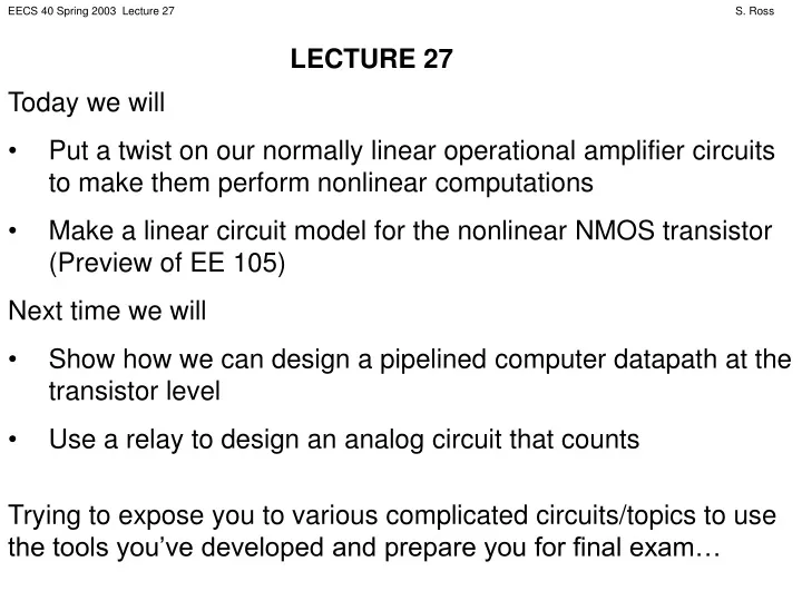
LECTURE 27 • Today we will • Put a twist on our normally linear operational amplifier circuits to make them perform nonlinear computations • Make a linear circuit model for the nonlinear NMOS transistor (Preview of EE 105) • Next time we will • Show how we can design a pipelined computer datapath at the transistor level • Use a relay to design an analog circuit that counts Trying to expose you to various complicated circuits/topics to use the tools you’ve developed and prepare you for final exam…
VIN NONLINEAR OPERATIONAL AMPLIFIERS When I put a nonlinear device in an operational amplifier circuit, I can compute a nonlinear function. Consider the following circuit using the realistic diode model: R VOUT +
VIN NONLINEAR OPERATIONAL AMPLIFIERS R ID VOUT + Computes an exponential function of VIN !
VIN NONLINEAR OPERATIONAL AMPLIFIERS What if I switch the positions of the resistor and the diode (and make sure VIN≥ 0 V)? ID R VOUT + Computes a natural logarithm function of VIN ! Changing the position of the elements inverted the function performed!
+ _ + _ TRANSISTOR AS CURRENT SOURCE But this hides the fact that IDSAT depends on VGS; it is really a voltage-dependent current source! If VGS is not constant, the model fails. What if VGS changes? What if there is noise in the circuit? This circuit acts like a constant current source, as long as the transistor remains in saturation mode. Load D IDSAT VDD G IDSAT Load VGS S
THE EFFECT OF A SMALL SIGNAL ID If VGS changes a little bit, so does ID. VGS = 2.1 V VGS = 2 V VGS = 1.9 V VDS
THE SMALL-SIGNAL MODEL Let’s include the effect of noise in VGS. Suppose we have tried to set VGS to some value VGS,DC with a fixed voltage source, but some noise DVGS gets added in. VGS = VGS,DC + DVGS + VGS - D G IDSAT,DC = f(VGS,DC) DIDSAT = g(DVGS) S We get the predicted IDSAT,DC plus a change due to noise, DIDSAT. No current flows into or out of the gate because of the opening.
THE SMALL-SIGNAL MODEL To be even more accurate, we could add in the effect of l. When l is nonzero, ID increases linearly with VDS in saturation. We can model this with a resistor from drain to source: + VGS - D G ro IDSAT,DC = f(VGS,DC) DIDSAT = g(DVGS) S The resistor will make more current flow from drain to source as VDS increases.
THE SMALL-SIGNAL MODEL How do we find the values for the model? IDSAT,DC = ½ W/L mN COX (VGS,DC – VTH)2 This is a constant depending on VGS,DC. This is a first-order Taylor series approximation which works out to DIDSAT = W/L mN COX (VGS,DC – VTH)DVGS We often refer to W/L mN COX (VGS,DC – VTH) as gm, so DIDSAT = gmDVGS.
THE SMALL-SIGNAL MODEL Including the effect of l via ro, the added current contributed by the resistor is Ir0 = ½ W/L mN COX (VGS – VTH)2lVDS To make things much easier, since the l effect is small anyway, we neglect the effect of DVGS in the resistance, so the current is Ir0≈ ½ W/L mN COX (VGS,DC – VTH)2lVDS = IDSAT,DCl VDS This leads to r0 = VDS / Ir0 = (l IDSAT,DC)-1
1.5 kW D ID + VDS _ 4 V G + VGS _ 3 V + _ + _ S EXAMPLE Revisit the example of Lecture 20, but now the 3 V source can have noise up to ± 0.1 V. Find the range of variation for ID. VTH(N) = 1 V, W/L mnCOX = 500 m A/V2, l = 0 V-1. We figured out that saturation is the correct mode in Lecture 20. The “noiseless” value of ID is IDSAT,DC = ½ W/L mN COX (VGS,DC – VTH)2 = 250 mA/V2 (3 V – 1 V)2 = 1 mA
1.5 kW D ID + VDS _ 4 V G + VGS _ 3 V + _ + _ S EXAMPLE The variation in ID due to noise: DIDSAT = W/L mN COX (VGS,DC – VTH)DVGS = 500 mA/V2 (3 V – 1 V) 0.1 V = 100 mA So ID could vary between 1.1 mA and 0.9 mA. Will saturation mode be maintained? Yes.