Download
1 / 42
420 likes | 565 Views
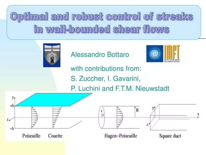
ROUTES TO TRANSITION IN SHEAR FLOWS. Optimal and robust control of streaks in wall-bounded shear flows. Alessandro Bottaro with contributions from: S. Zuccher, I. Gavarini, P. Luchini and F.T.M. Nieuwstadt.

E N D
ROUTES TO TRANSITION IN SHEAR FLOWS Optimal and robust control of streaks in wall-bounded shear flows Alessandro Bottaro with contributions from: S. Zuccher, I. Gavarini, P. Luchini and F.T.M. Nieuwstadt
1.TRANSITION IN SHEAR FLOWS IS A PHENOMENON STILL NOT FULLY UNDERSTOOD. For the simplest parallel or quasi-parallel flows there is poor agreement between predictions from the classical linear stability theory (Recrit) and experimentals results (Retrans)PoiseuilleCouette Hagen-Poiseuille BlasiusRecrit 5772 ~ 500Retrans ~ 1000 ~400 ~2000 ~400
2.TRANSITION IN SHEAR FLOWS IS A PHENOMENON STILL NOT FULLY UNDERSTOOD.
THE TRANSIENT GROWTH • THE MECHANISM: a stationary algebraic instability exists in the inviscid system (“lift-up” effect). In the viscous case the growth of the streaks is hampered by diffusion transient growth P.H. Alfredsson and M. Matsubara (1996); streaky structures in a boundary layer. Free-stream speed: 2 [m/s], free-stream turbulence level: 6%
Proposition: Optimal and robust control of streaks during their initial development phase, in pipes and boundary layers by • acting at the level of the disturbances (“cancellation control”) • acting at the level of the mean flow (“laminar flow control”)
Optimal cancellation control of streaks Cancellation Control Known base flow U(r); disturbance O(e) control O(e) Disturbance field (system’s state) Control O(e)
Optimal laminar flow control of streaks Laminar Flow Control Compute base flow O(1) together with the disturbance field O(e) control O(1) Whole flow field (system’s state) Control O(1)
OPTIMAL CONTROL: A PARABOLIC MODEL PROBLEM ut + uux = uxx + S u(t,x): state of the system u(0,x)=u0(x) u0(x): initial condition u(t,0)=uw(t) uw(t): boundary control u(t,)=0 S(t,x): volume control Suppose u0(x) is known; we wish to find the controls, uw and S, that minimize the functional: I(u, uw, S) = u2 dt dx + a2 uw2 dt + b2 S2 dt dx disturbance norm energy needed to control
I(u,uw,S) = u2 dt dx + a2 uw2 dt + b2 S2 dt dx a=b=0no limitation on the cost of the control aand/orb smallcost of employing uw and/or S is not important aand/orb largecost of employing uw and/or S is important
Optimal control For the purpose of minimizing I, let us introduce an augmented functional L = L(u,uw,S,a,b), with a(t,x) and b(t) Lagrange multipliers, and let us minimize the new objective functional L(u, uw, S, a, b) = I + a (ut + uux - uxx - S) dt dx + + b(t) [u(t,0)-uw(t)] dt Constrained minimization of I Unconstrained minimization of L
Optimal control Each directional derivative must independently vanish for a relative minimum of L to exist. For example it must be:
Optimal control Since du is an arbitrary variation, the double integral vanish if and only if the linear adjoint equation at + uax = - axx + 2u is satisfied, together with: a(T,x)=0 terminal condition a(t,0)=a(t,)=0 boundary conditions The vanishing of the other directional derivatives is accomplished by letting:
Optimal control Resolution algorithm: direct equations for state u (using uwand S) convergence test optimality conditions: uw(t)=ax(t,0)/2a2 S(t,x)=a(t,x)/2b2 adjoint equations for dual state a Optimality conditions are enforced by employing a simple gradient or a conjugate gradient method
ROBUST CONTROL: A PARABOLIC MODEL PROBLEM ut + uux = uxx + S u(t,x): state of the system u(0,x)=u0(x) u0(x): initial condition u(t,0)=uw(t) uw(t): boundary control u(t,)=0 S(t,x): volume control Now u0(x) is not known; we wish to find the controls, uw and S, and the initial condition u0(x) that minimize the functional: I1(u, u0,uw, S) = u2 dt dx + a2 uw2 dt + b2 S2 dt dx - - g2 u02 dx i.e. we want to maximize over all u0.
Robust control This non-cooperative strategy consists in finding the worst initial condition in the presence of the best possible control. Procedure: like previously we introduce a Lagrangian functional, including a statement on u0 L1(u, u0, uw, S, a, b, c) = I1 + a (ut + uux - uxx - S) dt dx + b(t) [u(t,0)-uw(t)] dt + c(x) [u(0,x)-u0(x)] dx
Robust control 2g2u0(x)=a(0,x) Vanishing of yields: 2g2u0(x)=a(0,x) Robust control algorithm requires alternating ascent iterations to find u0 and descent iterations to find uw and/or S. Convergence to a saddle point in the space of variables.
Optimal cancellation control of streaks Optimal control of streaks in pipe flow Spatially parabolic model for the streaks: structures elongated in the streamwise direction x Long scale for x: R Re Short scale for r:R Fast velocity scale for u: Umax Slow velocity scale for v, w: Umax/Re Long time: R Re/Umax
Optimal cancellation control of streaks Optimal control of streaks in pipe flow with
Optimal cancellation control of streaks with with
Optimal disturbance at x=0 Initial condition for the state: optimal perturbation, i.e. the disturbance which maximizes the gain G in the absence of control.
Optimal cancellation control of streaks Optimal control with where is the control statement =
Optimal cancellation control of streaks Order of magnitude analysis: Equilibrium increases Small increases Flat increases Cheap
Optimal cancellation control of streaks As usual we introduce a Lagrangian functional, we impose stationarity with respect to all independent variables and recover a system of direct and adjoint equations, coupled by transfer and optimality conditions. The system is solved iteratively; at convergence we have the optimal control.
Optimal and robust cancellation control of streaks • In theory it is possible to optimally counteract disturbances • propagating downstream of an initial point • (trivial to counteract a mode) • Physics: role of buffer streaks • Robust control laws are available • Next: • Feedback control, using the framework recently • proposed by Cathalifaud & Bewley (2004) • Is it technically feasible?
Optimal laminar flow control of streaks Optimal control of streaks in boundary layer flow Spatially parabolic model for the streaks: steady structures elongated in the streamwise direction x Long scale for x: L Short scale for y and z:d = L/Re Fast velocity scale for u: U Slow velocity scale for v, w: U /Re
Optimal laminar flow control of streaks Optimal control of streaks in boundary layer flow with
Optimal laminar flow control of streaks : : with the Gain given by:
Optimal laminar flow control of streaks Lagrangian functional: Stationarity of Optimality system
Optimal laminar flow control of streaks __________
Optimal and robust laminar flow control of streaks • Mean flow suction can be found to optimally damp the • growth of streaks in the linear and non-linear regimes • Both in the optimal and robust control case the control • laws are remarkably self-similar Bonus for applications • No need for feedback • Technically feasible (cf. ALTTA EU project)
Conclusions • Optimal control theory is a powerful tool • Robust control strategies are available through the direct- • adjoint machinery • Optimal feedback control is under way • Optimal control via tailored magnetic fields should be feasible