Pattern Recognition: Baysian Decision Theory

Pattern Recognition:Baysian Decision Theory Charles Tappert Seidenberg School of CSIS, Pace University

Pattern ClassificationMost of the material in these slides was taken from the figures in Pattern Classification (2nd ed) by R. O. Duda, P. E. Hart and D. G. Stork, John Wiley & Sons, 2001

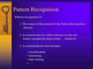
Baysian Decision Theory • Fundamental pure statistical approach • Assumes relevant probabilities are known perfectly • Makes theoretically optimal decisions

Baysian Decision Theory • Based on Bayes formula P(j| x) = p(x | j)P(j) / p(x) which is easily derived from writing the joint probability density two ways • P(j , x) = P(j|x)p(x) • P(j , x) = p(x|j)p(j) Note: uppercase P(.) denotes a probability mass function and lowercase p(.) a density function

Bayes Formula • Bayes formula P(j| x) = p(x | j)P(j) / p(x) can be expressed informally in English as posterior = likelihood x prior / evidence and Bayes decision chooses the class j with the greatest posterior probability

Bayes Formula • Bayes formula: P(j| x) = p(x | j)P(j) / p(x) • Bayes decision chooses class j with the greatest P(j| x) • Since p(x)is the same for all classes, greatest P(j| x) means greatest p(x | j)P(j) • Special case: if all classes are equally likely, i.e. same P(j), we get a further simplification – greatest P(j| x) is greatest likelihood p(x | j)

Baysian Decision Theory • Now, let’s look at the fish example of two classes – sea bass and salmon – and one feature – lightness • Let p(x | 1) and p(x | 2) describe the difference in lightness between populations of sea bass and salmon (see next slide)

Baysian Decision Theory • In the previous slide, if the two classes are equally likely, we get the simplification – greatest posterior means greatest likelihood,and Bayes decision is to choose class 1 when p(x | 1) > p(x | 2), i.e. when lightness is > approximately 12.4 • However, if the two classes are not equally likely, we get a case like the next slide

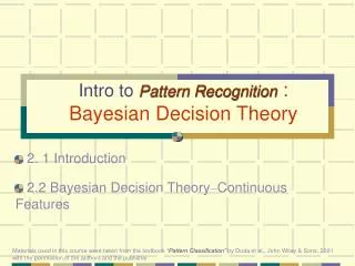
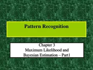
Baysian Parameter Estimation • Because the actual probabilities are rarely known, they are usually estimated after assuming the form of the distributions • The usually assumed form of the distributions is multivariate normal

Baysian Parameter Estimation • Assuming multivariate normal probability density functions, it is necessary to estimate for each pattern class • Feature means • Feature covariance matrices

Multivariate Normal Densities • Simplifying assumptions can be made for multivariate normal density functions • Statistically independent features with equal variances yields hyperplane decision surfaces • Equal covariance matrices for each class also yields hyperplane decision surfaces • Arbitrary normal distributions yields hyperquadric decision surfaces

Nonparametric Techniques • Probabilities are not known • Two approaches • Estimate the density functions from sample patterns • Bypass probability estimation entirely • Use a non-parametric method • Such as k-Nearest-Neighbor

k-Nearest-Neighbor

k-Nearest-Neighbor (k-NN) Method • Used where probabilities are not known • Bypasses probability estimation entirely • Easy to implement • Asymptotic error never worst than twice Baysian error • Computationally intense, therefore slow

Simple PR System with k-NN • Good for feasibility studies – easy to implement • Typical procedural steps • Extract feature measurements • Normalize features to 0-1 range • Classify by k nearest neighbor • Using Euclidean distance

Simple PR System with k-NN (cont):Two Modes of Operation • Leave-one-out procedure • One input file of training/test patterns • Repeatedly train on all samples except one which is left for testing • Good for feasibility study with little data • Train and test on separate files • One input file for training and one for testing • Good for measuring performance change when varying an independent variable (e.g., different keyboards for keystroke biometric)

Simple PR System with k-NN (cont) • Used in keystroke biometric studies • Feasibility study – Dr. Mary Curtin • Different keyboards/modes – Dr. Mary Villani • Used in other studies that used keystroke data • Study of procedures for handling incomplete and missing data – e.g., fallback procedures in the keystroke biometric system – Dr. Mark Ritzmann • New kNN-ROC procedures – Dr. Robert Zack • Used in other biometric studies • Mouse movement – Larry Immohr • Stylometry + keystroke study – John Stewart

Conclusions • Bayes decision method best if probabilities known • Bayes method okay if you are good with statistics and the form of the probability distributions can be assumed, especially if there is justification for simplifying assumptions like independent features • Otherwise, stay with easier to implement methods that provide reasonable results, like k-NN

Pattern Recognition: Baysian Decision Theory