Download
1 / 37
380 likes | 528 Views
Modeling Cyclical Growth. Steve Keen School of Economics & Finance University of Western Sydney. The Project. UNEP specification of non-equilibrium economic model Linked to CSIRO bio-physical model My brief: Take single sectoral model of cycles (Keen 1995 etc.)

E N D
Modeling Cyclical Growth Steve Keen School of Economics & Finance University of Western Sydney
The Project • UNEP specification of non-equilibrium economic model • Linked to CSIRO bio-physical model • My brief: • Take single sectoral model of cycles (Keen 1995 etc.) • Single sectoral model of credit (Keen 2009 etc.) • Combine into multi-sectoral cyclical model of credit and production • Never previously done • Previous attempts at dynamic “IO” input-output (multi-sectoral) models generally failed • Fatal instabilities—negative prices etc. • No previous attempts to model multisectoral monetary dynamics
Trends in economic data • Growth the norm in market economies...
Cycles in economic data • As are cycles... • Previous data, de-trended:
Conventional economic models • “Neoclassical” General Equilibrium models • Focus on trend • Ignore cycles • Ignore money • Presume system is • In equilibrium unless “shocked” • Will return to equilibrium after “exogenous shock” • Yet models have “dual instability” dilemma • Prices or quantities or both must be unstable • Effectively a barter system • Money only affects relative prices & inflation • Cycles assumed to be caused by noneconomic factors • Agriculture/weather/sunspots... (meteors?)
Conventional economic models • “The capitalistic economy is stable, and absent some change in technology or the rules of the economic game, the economy converges to a constant growth path with the standard of living doubling every 40 years.” • Edward C. Prescott (Nobel Prize 2004 for Real Business Cycle Theory), 1999 • “As ... discussed in ... “The Dynamic General Equilibrium Model,” the model features a representative household [i.e., one only!] that chooses paths of consumption, leisure, and investment to maximize utility. The paths of TFP and population are exogenously given, and the agent has perfect foresight over their values. We start the model at date T0 = 1980 and let time run out to infinity...” Conesa 2007
Conventional economic models • “The model could be described as broadly new Keynesian in its dynamic structure but with an equilibrating long run. • Activity is demand determined in the short run but supply determined in the long run… • The model will eventually return to a supply determined equilibrium growth path in the absence of demand or other shocks.” • Australian Treasury TRYM Model (2001) • Cycles treated as exogenous to model of economy...
Conventional economic models • E.g. unemployment in Australian Treasury TYRM model • History taken as given • Convergence to equilibrium assumed • Equilibrium long run growth rate assumed
Conventional economic models • Treatment of money and debt • In general, money ignored • “One thing which has not changed over the past five years is the philosophy underpinning the model. • It remains small, highly aggregated, empirically based, and non-monetary in nature.” Australia’s RBA (2005) • Money “neutrality” assumed • Affects price level but not real output • Universally, private debt ignored • Versus empirical data...
Endogenous Money • “The fact that the transaction component of real cash balances (M1) moves contemporaneously with the cycle • while the much larger nontransaction component (M2) leads the cycle • suggests that credit arrangements could play a significant role in future business cycle theory. • Introducing money and credit into growth theory in a way that accounts for the cyclical behavior of monetary as well as real aggregates is an important open problem in economics.” • Kydland and Prescott (1990, p. 15. Emphasis added) • 1990 analysis confirmed by more recent data • E.g., leads and lags for Australia 1954-2009:
Endogenous Money • Credit leads cycle with significant correlation • All other variables lag or have low correlations:
Key role of private debt • “Our tests produce a clear story about short-term financing decisions in response to earnings and investment... • The leverage and debt regressions then confirm that, for dividend payers, debt is indeed the residual variable in financing decisions. • Like dividend payers, non-payers primarily use debt to absorb short-term variation in earnings and investment.” (Fama & French 2000; emphases added)
Objectives for our economic model • Non-equilibrium • Economy itself inherently & endogenously cyclical • Model had to represent this • Multi-sectoral • Many non-neoclassical endogenous cycle models • But none to date were multi-sectoral • Explicitly monetary • Key role of money & debt shown in data • Incorporate interplay of debt, money and cycles • 3 key foundations • Goodwin “Growth Cycle” model (1967) • Minsky “Financial Instability Hypothesis” • Graziani “Circuit Theory” model of credit creation
Foundations (1) Cycles: Goodwin’s “Growth Cycle” • Capital K determines output Y via the accelerator: • Y determines employment L via productivity a: • L determines employment rate l via population N: • l determines rate of change of wages w via P.C. • Integral of w determines W (given initial value) • Y-W determines profits P and thus Investment I… • Closes the loop:
Foundations (1) Cycles: Goodwin’s “Growth Cycle” • Goodwin’s“Lokta-Volterra” model generates cycles: • Cycles caused by essential nonlinearity: • Wage rate times employment • Behavioural nonlinearities not needed for cycles; • Instead, restrain values to realistic levels
Foundations (2) Debt: Minsky’s “FIH” • Only theory that predicts this financial crises: • “it is necessary to have an economic theory which makes great depressions one of the possible states in which our type of capitalist economy can find itself.” (Can "It” Happen Again? A Reprise) • Time-&-debt-aware model: • Economy in historical time • Debt-induced recession in recent past • Firms and banks conservative re debt/equity, assets • Only conservative projects are funded • Recovery means most projects succeed • Firms and banks revise risk premiums • Accepted debt/equity ratio rises • Assets revalued upwards…
Foundations (2) Debt: Minsky’s “FIH” • Period of tranquility causes expectations to rise… • “Stability—or tranquility—in a world with a cyclical past and capitalist financial institutions is destabilizing.” (The Financial Instability Hypothesis: A Restatement) • Self-fulfilling expectations • Decline in risk aversion causes increase in investment • Investment expansion causes economy to grow faster • Asset prices rise • speculation on assets profitable • Increased willingness to lend increases money supply • Money supply endogenous money, not under Fed control • Riskier investments enabled, asset speculation rises • The emergence of “Ponzi” financiers • Cash flow less than debt servicing costs • Profit by selling assets on rising market • Interest-rate insensitive demand for finance
Foundations (2) Debt: Minsky’s “FIH” • Eventually: • Rising rates make conservative projects speculative • Non-Ponzi investors sell assets to service debts • Entry of new sellers floods asset markets • Rising trend of asset prices falters or reverses • Ponzi financiers go bankrupt: • Can no longer sell assets for a profit • Debt servicing on assets far exceeds cash flows • Asset prices collapse, increasing debt/equity ratios • Endogenous expansion of money supply reverses • Investment evaporates; economic growth slows • Economy enters a debt-induced recession • Back where we started...
Foundations (3): Endogenous money • Fundamental Endogenous Money insight • “Loans create Deposits” • Reverse of “Money Multiplier” model • Suggested directly modeling bank credit creation via account dynamics • Simple model of “Wicksellian” pure credit economy • No government sector or fiat money (yet) • Explicitly monetary model • “Double-entry book-keeping” meets symbolic math
Foundations (3): Endogenous money New methodology for dynamic modelling Table where each column represents a stock Each row represents relations between system states… Relations Equations • To generate the model, symbolically add up each column • Sum of column is differential equation for stock • Continuous time, not “discrete” time • Strictly monetary model of pure credit multi-commodity production economy developed…
Foundations (3): Endogenous money Input system as table: Interest flows: bank<―>firm Wage flows: firm―>workers Interest flows: bank―>workers Consumption flows: bank & workers―>firms Debt repayment flows: firms―>bank Reserve relending flows: bank―>firms New Money/Debt flows: bank<―>firms • Symbolic substitutions for placeholders above: • E.g., A is “loan interest rate times outstanding debt” • Time lags used for behavioural variables
Foundations (3): Endogenous money • Simple code develops mode automatically: Over to Mathcad…
Modelling a Credit Crunch • Simple production model linked to financial flows • Output is Labour times productivity • Labour is Money Wages flow divided by Money Wage rate • Wage set by Phillips curve unemployment-money wage change function • Price (necessary link between $ accounts and physical output) lagged convergence to markup over monetary cost of production • Single sectoral model generates stable dynamics • Can be used to consider some policy questions • But no cycles as yet • Policy example—stimulus to overcome credit crunch
Modelling a Credit Crunch • What’s better? Stimulus to lenders or debtors? • Injected into either BR (Bank Reserves) or FD (Firm Deposits) in simulation • Stimulus far more effective if given to debtors
Producing a multi-sectoral nonequilibrium model • Minsky model • Goodwin cycles • Debt “ratchets up” of in series of cycles • With “Ponzi lending”, tends towards Depression • But implicit money only (debt to GDP ratio) • Graziani model • Explicit money • Monetary determination of equilibrium output • But no cycles • Blending two models necessitates multi-sectoral model • Capital sector for purchases of investment goods • Easily built using “Table to Dynamic Model” technology
A Multi-sectoral monetary model • More complicated table (2 sector version shown here): • Capital and Consumer Goods Sectors • All sectors in 2 halves to force recording of intra-sectoral monetary purchases • Investment & inter-sectoral demand • Time lags are time-varying functions of rate of profit rather than constant parameters
A Multi-sectoral monetary model • More complex financial model results • Constrained by nonlinear behavioural relations • (Nonlinear functions not essential for dynamics but constrain simulation values to more realistic ranges)
A Multi-sectoral monetary model • Allied to lagged Goodwin growth cycle production model • Investment minus Depreciation determines Capital • Output function of capital stock • Employment function of output • Model of financially driven cyclical economy • Simulations shown here lead to sustained cycles • (No speculative debt in model as yet) • Overall system very complex • But easily simulated in modern software • Scales indefinitely (more sectors easily added)
A Multi-sectoral monetary model • Model requires minimum of • 4n+3 financial ODEs • 2n Loan & 2n Deposit • Bank Income • Bank Reserves • Household Deposit • 5n sectoral equations • capital, output, labour, prices, productivity • 1 population equation • 40 ODEs in this 4 sector model
A Multi-sectoral monetary model • Notional Sectors in system shown here: • Capital Goods • Consumer Goods • Agriculture • Energy • Generates complex endogenous cycles in income shares, output, credit, employment—just like actual economy • No need for “exogenous shocks” • Though can also be added in future • Not yet fitted to empirical data • But qualitative behaviour of model matches “stylised facts” of (credit-driven) business cycle
A Multi-sectoral monetary model of production • Endogenous cycles... • Cycles similar to stylised facts of business cycle • Long accelerating boom • Sudden slump • Tepid recovery before next boom
A Multi-sectoral monetary model of production • With equilibrium models • History cyclical • The future equilibrium... • With non-equilibrium model, projections look like history • Cycles in past & future
A Multi-sectoral monetary model of production • Crucial role of credit • Change in credit leads cycle
A Multi-sectoral monetary model of production • Income distribution cycles...
A Multi-sectoral monetary model of production • Crucial role of monetary variables • Simulation show here generates “stable instability” • Cycles but not breakdown • Different parameters can generate • Convergence to stability; or • Financial collapse (Great Depression)
A Multi-sectoral monetary model of production • Crucial characteristic that cycles are endogenous • General Disequilibrium as hallmark of a good model • “Instability is an observed characteristic of our economy. • For a theory to be useful as a guide to policy for the control of instability, the theory must show how instability is generated. • The abstract model of the neoclassical synthesis cannot generate instability...” • (Minsky, “Can "It“ Happen Again? A Reprise”)
Future development of model • First “meteorological” model of capitalism • Causal dynamics rather than equilibrium assumptions • Realistic non-equilibrium multi-sectoral production • Designed for rising realism/complexity over time • Parameter calibration of nonlinear, disequilibrium model • Two approaches to data fitting feasible • Fit functions and selected empirical data • Fit overall model and generate realistic nonlinear functions, lags, etc. from that • Develop to generate alternative scenarios • All will include cyclical, non-equilibrium future • Enable automatic generation of higher-dimensional multisectoral models