Download
1 / 33
350 likes | 536 Views
Supply Chain Dynamics and Forecasting. Presenter: Mu Niu. The Context. Companies make huge investments in Manufacturing Resource Planning systems . However, even with the introduction of resource planning systems, the performance of the supply chain remains problematic ( Lyneis, 2005 ).

E N D
Supply Chain Dynamics and Forecasting Presenter: Mu Niu
TheContext • Companies make huge investments in Manufacturing Resource Planning systems. However, even with the introduction of resource planning systems, the performance of the supply chain remains problematic( Lyneis, 2005 ). • They do not take into account the inherent ‘messiness’ of situations that contain human decision making within the process. • Such tools do not promote learning or effective decision support as they do not include the powerful technique of simulation to allow for what-if analysis of alternative strategies . Page 2 Dynamics and Forecasting 31/07/2014
The Problem • A centralised supply chain system was recently implemented in Draeger Safety Ltd, with the purpose of diminishing costs and avoiding backlogs. However, the central Hub in Germany still hold big amount of inventory. • This made Draeger’s planning managers even more worried as it was difficult to predict what the consequences of centralised inventories would be for the manufacturing plant in Blyth. Page 3 Dynamics and Forecasting 31/07/2014
TheResearch Focus • Modelling and simulation of the material and information flows including the decision processes of the centralised supply-chain at Draeger Safety, UK; • Analyses of the behaviour of inventories with relation to different decision strategies and characteristics of managers; • Evaluate the sensitivity of the supply chain to different methods of forecasting; • Develop a Microworld (Senge, 1990) to enable managers to conduct what-if scenarios and learn about the behaviour of the supply chain. Page 4 Dynamics and Forecasting 31/07/2014
China Hub Asia Singapore Japan Goods Shipped Order in France Central Hub Germany Order in Factory Blyth UK Denmark Goods Shipped Goods Shipped Order in USA Hub USA Canada Draeger supply chain structure Page 5 Dynamics and Forecasting 31/07/2014
1Month M’facture Germany Primary Hub Blyth Factory Hub Sales Horders Hub Forecast Hforecast Hub Requirement Hreq Production Fprod Backlog Hblk Backlog Fblk Hub Shipments Hship Factory Shipments Fship Inventory Hinv Inventory Finv 1Month T’ Delay Germany- UK Model Page 6 Dynamics and Forecasting 31/07/2014
Model Equations • Hinv(t) = max(0, Hinv(t-1) + Fship(t-1) – Hship(t)) • Hblk(t) = max(0, Hblk(t-1) + Horders(t) - (Hinv(t-1) + Fship(t-1)); HUB • Hship(t) = min(Horders(t) + Hblk(t-1), Hinv(t-1) + Fship(t-1)); • Finv(t) = max(0, Finv(t-1) + Fprod(t-1) – Fship(t)) • Fblk(t) = max(0, Fblk(t-1) + Hreq(t+1) - (Finv(t-1) + Fprod(t-1)); Factory • Fship(t) = min(Hreq(t+1) + Fblk(t-1), Finv(t-1) + Fprod(t-1)); • Hforcast(t+2) = (1 - θ) Horders(t) + θ Hforcast(t+1); • Hreq(t+2) = max( 0, α( Q – Hinv(t) + Hblk(t) ) –αβ( Fblk(t) +Fship(t) )+ Hforcast(t+2)); Decision • Fprod(t) = max( 0, α ( Q – Finv(t) + Fblk(t) ) + Hreq(t+2) ) Making α, is a measure of the aggressiveness with which inventory differences are corrected. [0,1] β, is a measure of the weight with which inventory ordered but still to arrive. [0,1] Page 7 Dynamics and Forecasting 31/07/2014
Time simulation Stable Limit cycle Quasi periodic Chaotic
Equations X(k) = A X(k-1) + B U(k)
System Block Diagram Page 11 Dynamics and Forecasting 31/07/2014
Eigenvalues plotted for α = 0:0.01:1 , β = 0 and β = 0:0.01:1 , α = 1 with unit circle α = 0:0.01:1 , β = 0 β = 0:0.01:1 , α = 1 Page 12 Dynamics and Forecasting 31/07/2014
The stability analysis • For the condition β = 0 (depicted in Figure of eigenvalue plots), the Factory characteristic equation is: • (z + α)(z -1) + α = 0 • This has two eigenvalues, one at z = 0 and a second, which is always real and which lies in the range z = 1 → 0 as α = 0 → 1. • The Hub characteristic equation is: • (z2 + α)(z -1) + α = 0 • This has three eigenvalues. Again one of these is at z = 0, the other two form a second order pair that become complex when α > 0.25. It is this pair that is clearly identified in Figure of eigenvalue plots. • Moreover, it is the Hub’s dynamics and not the Factory’s that are the potential source of unstable behavior. The Hub, potentially, becoming unstable for any value of α > 1, (whilst the Factory would be stable for any value of α < 2.) Page 13 Dynamics and Forecasting 31/07/2014
Model with two additional Production delays To explore the long lead time production dynamics. The additional delay were added into the production Page 14 Dynamics and Forecasting 31/07/2014
Eigenvalues plotted for α = 0:0.01:1 , β = 0 and β = 0:0.01:1 , α = 1 with unit circle
Model Analysis • analysis given that the replenishing inventory rate α has a destablising effecs while the consideration of the past decision rate β has a stablising effects on the dynamics of this production delayed supply chain model. • The extra production delay has made the system more sensitive to the management decisions. Comparing with the original model, the production delay model could be unstable, even the eigenvalues locating inside of the unit circle. • managers have a flexible option by improving the safety stock Q to stabilize the supply chain and achieve the on time delivery. However the warehouse has to pay more costs for holding the extra mount of safety stock. • With the introduction of the two additional lead time states, it is the Factory which provide the primary route toward instablility. In this situation, the Hub can do little about the poor management decisions in the Factory. Page 17 Dynamics and Forecasting 31/07/2014
Model with an Planning delays • The planning delay represents two likely scenarios • Getting forecast wrong • Compatibility problems between the planning systems at different locations Page 18 Dynamics and Forecasting 31/07/2014
System block diagram Hub Factory
Eigenvalues plotted for α = 0:0.01:1 , β = 0 and β = 0:0.01:1 , α = 1 with unit circle
Model Analysis • Just as in the two previous cases, α has a destabilising influence whilst β is stabilising. • For this situation it is again the Hub management policy that is the primary route to instability. However, with the additional information delay the Hub’s route to instability now follows the more severe path. • In the presence of the one month information delay, even the stabilising influence of β only lessens the severity of the route to instability. As long as α =1, no matter what β is, the model is always oscillating. Operations on the safety stock Q cannot make effects for the unstable behavior. • Thus, for this situation good management and management policies are critical if significant problems are to be avoided. Therefore, the accurate forecasting is essential to improve the supply chain performance. Page 21 Dynamics and Forecasting 31/07/2014
Time series Prediction • The basic principle of time series prediction is to use a model to predict the future data based on known past data. • Many kinds of forecasting methods implemented withsystem dynamic approach,ARMA (auto-regression and moving average) model, wavelet neural networks model has been applied. • A performance function, which measures the absolute difference between forecast and real data, is employed to record the cost for each different structured model ; Page 22 Dynamics and Forecasting 31/07/2014
The original data • The original data is 64 months sales history of Lung demand valve Page 23 Dynamics and Forecasting 31/07/2014
ARMA withoutany preprocessing The coefficient is produced and updated by Recursive least square Page 24 Dynamics and Forecasting 31/07/2014
ARMA with Differencing preprocessing Page 25 Dynamics and Forecasting 31/07/2014
Cost function Page 26 Dynamics and Forecasting 31/07/2014
NN1 Wavelet Threshold Decompose Reconstruct NN2 NN4 Prediction NN3 Wavelet Neural Networks This hybrid scheme includes three stages. 1)The time series were decomposed with a wavelet function into three sets of coefficients. 2) Three new time series is predicted by a separate NN; 3)The prediction results are used as the inputs of the third stage, where the next sample of is derived by NN4. Page 27 Dynamics and Forecasting 31/07/2014
Forecasting results ARMA Neural Network Page 28 Dynamics and Forecasting 31/07/2014
Cost function Page 29 Dynamics and Forecasting 31/07/2014
Summary and Contributions • The behaviors of Draeger supply chain model has been analyzed with different decision parameters. The small signal analysis shows that when the system behaves normally (no backlog) the factory and the hub are decoupled. • We identified the principle source of unstable behavior could be the factory or hub depnding on the operating condition. In the original model the route toward instability is via via the Hub management policy. With the introduction of the extra states (additional lead-time), it is the Factory which now provides the primary route toward instability .In the presence of one month planning delay, the Hub’s route to instability follows the more severe path. • Because the systems are ‘isolated’ poor management decisions in the Hub cannot be corrected by good decisions in the Factory • We have shown the most severe route to the instability come from the errors in forecasting. The wavelet neural network forecasting apparently offers to improvement over the Draeger current forecasting approach. Page 30 Dynamics and Forecasting 31/07/2014
Further Research • Include the dynamics of other Hubs • Look at different decision making in different Hubs • look for methods to further improve forecasting
Publication • Niu M.,Sice P.,French I., Mosekilde E., (2007): The Dynamics Analysis of Simplified Centralised Supply Chain, The Systemist Journal, Oxford, UK, Nov.2007. • Niu M.,Sice P.,French I., Mosekilde E., (2008): Explore the Behaviour of Centralised Supply Chain at Draeger Safety UK, International Journal of Information system and Supply Chain Management, USA, Jan. 2008 (print copy availibel in Dec 2008). • French I., Sice P., Niu M., Mosekilde E.,(2008): The Dynamic Analysis of a Simplified Centralised Supply Chain and Delay Effects, System Dynamic Conference, Athens, July.2008. • Sice P., Niu M., French I., Mosekilde E., (2008): The Delay Impacts on a Simplified Centralised Supply Chain, UK Systems Society Conference, Oxford, UK, Sep.2008. • Niu M, Sice P., French I., (2008): Nonlinear Forecasting Model, Northumbria Research Forum 2008, Newcastle upon Tyne, UK. Page 33 Dynamics and Forecasting 31/07/2014