Download
1 / 26
260 likes | 347 Views
Random non-local games. Andris Ambainis, Artūrs Bačkurs, Kaspars Balodis, Dmitry Kravchenko, Juris Smotrovs, Madars Virza University of Latvia. Non-local games. Bob. Alice. a. b. x. y. Referee. Referee asks questions a, b to Alice, Bob; Alice and Bob reply by sending x, y;

E N D
Random non-local games Andris Ambainis, Artūrs Bačkurs, Kaspars Balodis, Dmitry Kravchenko, Juris Smotrovs, Madars Virza University of Latvia
Non-local games Bob Alice a b x y Referee Referee asks questions a, b to Alice, Bob; Alice and Bob reply by sending x, y; Alice, Bob win if a condition Pa, b(x, y) satisfied.
Example 1 Bob Alice a b x y Referee Winning conditions for Alice and Bob (a = 0 or b = 0) x = y. (a = b = 1) x y.
Example 2 Alice and Bob attempt to “prove” that they have a 2-coloring of a 5-cycle; Referee may ask one question about color of some vertex to each of them.
Example 2 Referee either: asks ith vertex to both Alice and Bob; they win if answers equal. asks the ith vertex to Alice, (i+1)st to Bob, they win if answers different.
Example 3 3-SAT formula F = F1 F2 ... Fm. Alice and Bob attempt to prove that they have x1, ..., xn: F(x1, ..., xn)=1.
Example 3 F = F1 F2 ... Fm. Bob Alice i j xj all xj, jFi Referee Referee chooses Fi and variable xj Fi. Alice and Bob win if Fi satisfied and xj consistent.
Non-local games in quantum world Bob Alice Corresponds to shared random bits in the classical case. • Shared quantum state between Alice and Bob: • Does not allow them to communicate; • Allows to generate correlated random bits.
Example:CHSH game Bob Alice a b x y Referee Winning condition: • (a = 0 or b = 0) x = y. • (a = b = 1) x y. Winning probability: • 0.75 classically. • 0.85... quantumly. A simple way to verify quantum mechanics.
Example: 2-coloring game Winning probability: • classically. • quantumly. Alice and Bob claim to have a 2-coloring of n-cycle, n- odd; 2n pairs of questions by referee.
Random non-local games Bob Alice a b x y Referee • a, b {1, 2, ..., N}; • x, y {0, 1}; • Condition P(a, b, x, y) – random; Computer experiments: quantum winning probability larger than classical.
XOR games • For each (a, b), exactly one of x = y and x y is winning outcome for Alice and Bob.
The main results • Let n be the number of possible questions to Alice and Bob. • Classical winning probability pcl satisfies • Quantum winning probability pq satisfies
Another interpretation • Value of the game = pwin – (1-pwin). Quantum advantage:
Comparison • Random XOR game: • CHSH game: • Best XOR game:
Methods: quantum Tsirelson’s theorem, 1980: • Alice’s strategy - vectors u1, ..., uN, ||u1|| = ... = ||uN|| = 1. • Bob’s strategy - vectors v1, ..., vN, ||v1|| = ... = ||vN|| = 1. • Quantum advantage
Random matrix question • What is the value of for a random 1 matrix A? Can be upper-bounded by ||A||=(2+o(1)) N √N
Lower bound • There exists u: • There are many such u: a subspace of dimension f(N), for any f(N)=o(N). Combine them to produce ui, vj:
Classical results Let n be the number of possible questions to Alice and Bob. Theorem Classical winning probability pcl satisfies
Methods: classical • Alice’s strategy - numbers u1, ..., uN {-1, 1}. • Bob’s strategy - numbers v1, ..., vN {-1, 1}. • Classical advantage
Classical upper bound • If Aij – random, Aijuivj – also random. • Sum of independent random variables; • Sum exceeds 1.65... N √N for any ui, vj, with probability o(1/4n). • 4N choices of ui, vj. • Sum exceeds 1.65... N √N for at least one of them with probability o(1).
Classical lower bound Given A, change signs of some of its rows so that the sum of discrepancies is maximized,
Greedy strategy • Choose u1, ..., uN one by one. k-1 rows that are already chosen 2 0 -2 ... 0 Choose the option which maximizes agreements of signs
Analysis 2 0 -2 ... 0 • On average, the best option agrees with fraction of signs. Choose the option which maximizes agreements of signs • If the column sum is 0, it always increases.
Rigorous proof 2 0 -2 ... 0 • Consider each column separately. Sum of values performs a biased random walk, moving away from 0 with probability in each step. Choose the option which maximizes agreements of signs • Expected distance from origin = 1.23... √N.
Conclusion • We studied random XOR games with n questions to Alice and Bob. • For both quantum and classical strategies, the best winning probability ½. • Quantumly: • Classically: