Download
1 / 32
320 likes | 437 Views
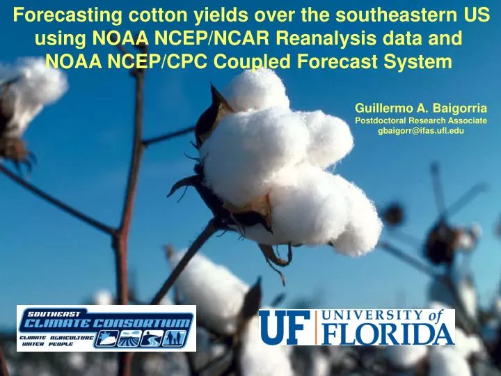
Forecasting cotton yields over the southeastern US using NOAA NCEP/NCAR Reanalysis data and NOAA NCEP/CPC Coupled Forecast System. Guillermo A. Baigorria Postdoctoral Research Associate gbaigorr@ifas.ufl.edu. (NCEP/CPC) (NCEP/CPC) (UF) (FSU/COAPS) (NCEP/CPC) (UM) (IRI) (IRI).

E N D
Forecasting cotton yields over the southeastern USusing NOAA NCEP/NCAR Reanalysis data and NOAA NCEP/CPC Coupled Forecast System Guillermo A. BaigorriaPostdoctoral Research Associate gbaigorr@ifas.ufl.edu
(NCEP/CPC) (NCEP/CPC) (UF) (FSU/COAPS) (NCEP/CPC) (UM) (IRI) (IRI) Muthuvel Chelliah Kingtse C. Mo James W. Jones James J. O’Brien R. Wayne Higgins Daniel Solis James W. Hansen Neil Wards
We developed a system potentially useful to forecast cotton yields in the SE-USA • Climate Test Bed provided us with new research partners
Cotton in the Southeast US • US$ 826 million (1997) in Alabama and Georgia (USDA/NASS) • In the last 30 years cotton increased by 800 thousand hectares in the US. • Much of this increase occurred in the Southeast where yields have also increased during this period • US cotton exports have more than doubled in the last 5 years • Sensible to plagues and diseases (i.e. Hardlock of cotton [Fusarium verticillioides]) reduced yields by about 50% in 2002 in the Panhandle of Florida
De-trended time series of cotton yields and ENSO phases(48-county average) El Niño Neutral Cotton yields (kg ha-1) La Niña
Cotton yield ENSO-based forecast Correlation ranges p< 0.00 r0.00 – 0.25 t0.25 – 0.50 v0.50 – 0.75 x0.75 – 1.00 no significant
What alternatives to ENSO do we have? Global/Regional Circulation Models (GCM/RCM) better predict the interannual climate variability and circulation patterns rather than the absolute values of meteorological variables.
DATA Climate data • NOAA NCEP/NCAR Reanalysis data (1970 – 2005) • NOAA NCEP/CPC Coupled Forecast System retrospective forecasts (1981-2005). Agricultural data • National Agricultural Statistics Service (NASS) 211 counties in Alabama (67), Florida (16) and Georgia (128) producing cotton. Only 48 counties were selected because of significant cotton production areas (35-year average ranging from 1,500 to 22,000 ha)
Cotton lint yields in Alabama and Georgia yields (kg ha-1) Most of the cotton in the southeastern US is planted between March and Apriland harvested between September and October
Goodness-of-Fit index (GFI) between observed rainfallat weather station and observed cotton yield anomalies G r o w t h F l o w e r i n g M a t u r i t y t o GFI = Average correlation over 48 counties
Relationship between humidity and cotton yield Under low to moderate rainfalland low atmospheric humidity Under moderate to high rainfalland high atmospheric humidity Hardlock of cotton Boll rot In the SE-USA this vulnerable-window period occurs during July and early August
Wind field anomalies at 200 hPa and SST anomalies Five years of highest yielding Five years of lowest yielding AMJ JAS Temperature anomaly
Surface temperatures Meridional winds at 200 hPa Correlation maps between de-trended cotton yields andNOAA NCEP/NCAR reanalysis data of: Reference: Baigorria, G.A., Hansen, J.W., Ward, N., Jones, J.W. and O’Brien, J.J. Assessing predictability of cotton yields in the Southeastern USA based on regional atmospheric circulation and surface temperatures. Journal of Applied Meteorology and Climatology. In press.
July – August - September Highest cotton yield Lowest cotton yield 200 hPa Temperatures lower than normalincrease air density producingsubsidence Temperatures higher than normaldecrease air density producingconvection 850 hPa Temperatures lower than normaldecrease absolute humidity,decreasing H2O available forcondensation Temperatures higher than normalincrease absolute humidity,increasing H2O available forcondensation Humid air Humid air convection convection Sfc. Land Ocean Land Ocean 850 hPa 200 hPa 850 hPa 200 hPa SST anomalies (°C)
°C Climatology 1981-2003 29 28 27 26 25 24 ObservedMean Temperaturesat Surface (July) Depending on cotton varieties, temperatures higher than 32°C cause boll abortion decreasing boll retention °C °C Highest yielding Lowest yielding 0 -0.2 -0.4 -0.6 -0.8 -1.0 0.8 0.6 0.4 0.2 0 -0.2 Anomalies °C Anomalies °C
W m-2 -12 -10 -8 -6 -4 -2 0 2 4 6 8 Observed anomalies of latent heat flux (July) Highest yielding Lowest yielding
Methods • Use as predictors the spatial structure of the NOAA NCEP/NCAR reanalysis 200 hPa meridional winds and surface temperatures from July to September captured by principal components • Use as predictors the spatial structure of the NOAA NCEP/CPC CFS 200 hPa meridional winds and surface temperatures from July to September captured by principal components • Applied canonical correlation analysis and leave-one-out cross-validation to predict the interannual variability of cotton yields in the 48 counties
Observed NCEP reanalysis-based prediction (cross-validated) NOAA NCEP/NCAR Reanalysis data All-county average Cotton lint yields (kg.ha-1) R = 0.6873 ** years 32 counties ** 15 counties * 1 county ns ** Significant at the 0.01 probability * Significant at the 0.05 probability
How this can support a farmer? • External symptoms of hardlock of cotton appear just previous to the harvest when there is nothing to do • Farmers usually do not apply fungicides because they don’t see the effects and they try to reduce costs • To wait for observed July data from NOAA NCEP/NCAR reanalysis will help farmers in early August to know if they will have harvest losses in November. It doesn’t help a lot, does it? • But what if at least we can forecast July conditions later June – early July (CFS 0-1 month in advance)? Farmers will have the information to help them in the decision whether applying fungicides just when the attack is beginning
500 hPa height anomalies during thehighest yielding years July Observed Climatology of 500 hPa height 500 hPa height anomalies during the lowest yielding years
PC of observed Z500 (NOAA NCEP/NCAR reanalysis) PC of observed cotton yields Canonical correlation July R = 0.9494
ENSO-based forecast Correlation ranges p< 0.00 r0.00 – 0.25 t0.25 – 0.50 v0.50 – 0.75 x0.75 – 1.00 no significant (based on 500 bootstrap samples, confidence level of 95%) NCEP Reanalysis-basedprediction (Cross-validated)
Observed NCEP reanalysis-based prediction (cross-validated) ENSO-based hindcasted All-county average RObs= 0.8744** RENSO= 0.2031ns Best estimated county Bleckley - Georgia Cotton lint yields (kg.ha-1) RObs= 0.8858** RENSO= - 0.2248ns Worst estimated county Mitchell - Georgia RObs= 0.6690** RENSO= 0.0979ns ** Significant at the 0.01 probability * Significant at the 0.05 probability Years
PC of CFS’s hindcasted circulation PC of observed cotton yields Canonical correlation July R = 0.7876
ENSO-based forecast Correlation ranges p< 0.00 r0.00 – 0.25 t0.25 – 0.50 v0.50 – 0.75 x0.75 – 1.00 no significant (based on 500 bootstrap samples, confidence level of 95%) CFS-based forecast (Cross-validated)
Observed CFS-based hindcasted (cross-validated) ENSO-based hindcasted All-county average RCFS= 0.7507** RENSO= 0.2031ns Best estimated county Terrell - Georgia Cotton lint yields (kg.ha-1) RCFS= 0.7879 ** RENSO= - 0.2745ns Worst estimated county Madison - Alabama RCFS= 0.4459 * RENSO= 0.2436ns ** Significant at the 0.01 probability * Significant at the 0.05 probability Years
Conclusions • Based on the previous almost total lack of predictability skills in the region during summertime, the method increased the probabilities to forecast cotton yields beyond the chances in up to 67%. • Specific atmospheric circulation patterns that favor higher humidity, temperatures and rainfall during summertime caused a tendency to lower cotton yields, which is consistent with boll abortion and higher than normal incidence of diseases during flowering and harvest. • In the case of predicting cotton yield, the dual effect of water during anthesis and boll maturity creates important challenges wherea multi-disciplinarily approach is the only way to tackle the issue.
Conclusions • It is necessary to go further in to investigate the physical relationship between the circulation patterns and the regional conditions where cotton are growing during summertime in the SE-USA. • It is necessary to analyze CFS’s forecasts made with more than one month in advance in order to assess the predictability levels with more time in advance.