Download
1 / 37
370 likes | 441 Views
Linear Classification with Perceptrons. Framework. Assume our data consists of instances x = ( x 1 , x 2 , ..., x n ) Assume data can be separated into two classes, positive and negative, by a linear decision surface .

E N D
Framework • Assume our data consists of instances x= (x1, x2, ..., xn) • Assume data can be separated into two classes, positive and negative, by a linear decision surface. • Learning: Assuming data isn-dimensional, learn (n−1)-dimensional hyperplaneto classify the data into classes.
Linear Discriminant Feature 1 Feature 2
Feature 2 Linear Discriminant Feature 1
Linear Discriminant Feature 1 Feature 2
Example where line won’t work? Feature 1 Feature 2
Perceptrons • Discriminantfunction: w0 is called the “bias”. −w0 is called the “threshold” • Classification:
Perceptrons as simple neural networks x1 x2 xn +1 w1 w0 w2 output . . . wn
Example • What is the class y? 1 -1 +1 .4 -.1 -.4
Hyperplane Geometry of the perceptron In 2d: Feature 1 Feature 2
In-class exercise Work with one neighbor on this: (a) Find weights for a perceptron that separates “true” and “false” in x1x2. Find the slope and intercept, and sketch the separation line defined by this discriminant. (b) What (if anything) might make one separation line better than another?
To simplify notation, assume a “dummy” coordinate (or attribute) x0 = 1. Then we can write:
Notation • Let S = {(xk, tk):k= 1, 2, ..., m}be a training set. xkis a vector of inputs: xk= (xk,1, xk,2, ..., xk,n) tkis {+1, −1} for binary classification, tk for regression. • Output o: • Error of a perceptron on the kth training example, (xk,tk)
Example • Training set: x1 = (0,0), t1 = −1 x2 = (0,1),t2 = 1 • Let w = {w0, w1, w2) = {0.1, 0.1, −0.3} What is E1? What is E2? +1 0.1 0.1 x1 o −0.3 x2
Coursepack is now (really!) on reserve at library Reading for next week: Coursepack: Learning From Examples, Section 7.3-7.5 (pp. 39-45). T. Fawcett, “An introduction to ROC analysis”, Sections 1-4, 7 (linked from the course web page)
f1 f2 f3 f4 f5 f6 f7 f8 Clarification on HW 1, Q. 2
Perceptrons (Recap) 1 w0 xi , wi w1 x1 output o inputx w2 x2 wn . . . xn
Perceptrons (Recap) 1 w0 xi , wi w1 x1 output o inputx w2 x2 wn . . . xn
Perceptrons (Recap) 1 w0 xi , wi w0 is called the “bias” −w0is called the “threshold” w1 x1 output o inputx w2 x2 wn . . . xn
Perceptrons (Recap) 1 w0 xi , wi w0 is called the “bias” −w0is called the “threshold” w1 x1 output o inputx w2 x2 wn . . . xn If then o = 1.
Notation Target value tis {+1, −1} for binary classification Error of a perceptron on the kth training example, (xk,tk):
How do we train a perceptron?Gradient descent in weight space From T. M. Mitchell, Machine Learning
Perceptron learning algorithm • Start with random weights w= (w1, w2, ... , wn). • Do gradient descent in weight space, in order to minimize error E: • Given error E, want to modify weights w so as to take a step in direction of steepest descent.
Gradient descent • We want to find w so as to minimize sum-squared error (or loss): • To minimize, take the derivative of E(w) with respect to w. • A vector derivative is called a “gradient”: E(w)
Here is how we change each weight: and is the learning rate.
Error function has to be differentiable, so output function o also has to be differentiable.
1 output -1 0 activation 1 output -1 0 activation Activation functions Not differentiable Differentiable
1 output -1 0 activation 1 output -1 0 activation Activation functions Approximate this With this Not differentiable Differentiable
This is called the perceptron learning rule, with “true gradient descent”.
Training a perceptron (true gradient descent) Assume there are m training examples and let be the learning rate (a user-set parameter). • Create a perceptron with small random weights, w = (w1, w2, ... , wn). • For k = 1 to m: Run the perceptron with input xkand weights wto obtain ok. • Go to 2.
Problem with true gradient descent: Training process is slow. Training process will land in local optimum. • Common approach to this: use stochastic gradient descent: • Instead of doing weight update after all training examples have been processed, do weight update after each training example has been processed (i.e., perceptron output has been calculated). • Stochastic gradient descent approximates true gradient descent increasingly well as 1/.
Training a perceptron(stochastic gradient descent) • Start with random weights, w= (w1, w2, ... , wn). • Select training example (xk, tk). • Run the perceptron with input xkand weights w to obtain ok. • Now, • Go to 2.
Perceptron learning rule: In-class exercise Training set: ((0,0), −1) ((0,1), 1) ((1,1), 1) Let w = {w0, w1, w2) = {0.1, 0.1,−0.3} +1 1. Calculate new perceptronweights after each training example is processed. Let η = 0.2 . 2. What is accuracy on training data after one epoch of training? Did the accuracy improve? 0.1 0.1 x1 o −0.3 x2
1960s: Rosenblatt proved that the perceptron learning rule converges to correct weights in a finite number of steps, provided the training examples are linearly separable. • 1969: Minsky and Papert proved that perceptrons cannot represent non-linearly separable target functions. • However, they proved that any transformation can be carried out by adding a fully connected hidden layer.
Multi-layer perceptron example Decision regions of a multilayer feedforward network. The network was trained to recognize 1 of 10 vowel sounds occurring in the context “h_d” (e.g., “had”, “hid”) The network input consists of two parameters, F1 and F2, obtained from a spectral analysis of the sound. The 10 network outputs correspond to the 10 possible vowel sounds. (From T. M. Mitchell, Machine Learning)
Good news: Adding hidden layer allows more target functions to be represented. • Bad news: No algorithm for learning in multi-layered networks, and no convergence theorem! • Quote from Minsky and Papert’s book, Perceptrons (1969): “[The perceptron] has many features to attract attention: its linearity; its intriguing learning theorem; its clear paradigmatic simplicity as a kind of parallel computation. There is no reason to suppose that any of these virtues carry over to the many-layered version. Nevertheless, we consider it to be an important research problem to elucidate (or reject) our intuitive judgment that the extension is sterile.”
Two major problems they saw were: • How can the learning algorithm apportion credit (or blame) to individual weights for incorrect classifications depending on a (sometimes) large number of weights? • How can such a network learn useful higher-order features? • Good news: Successful credit-apportionment learning algorithms developed soon afterwards (e.g., back-propagation). Still successful, in spite of lack of convergence theorem.