Download
1 / 16
320 likes | 983 Views
Chemical Mass Balance Model ( CMB8.2). A receptor model for assessing source apportionment using ambient data and source profile data with appropriate uncertainty estimates.

E N D
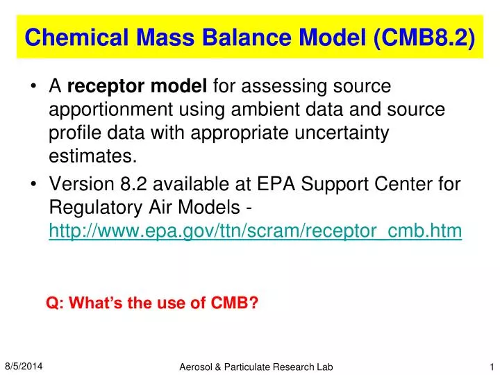
Chemical Mass Balance Model (CMB8.2) • A receptor model for assessing source apportionment using ambient data and source profile data with appropriate uncertainty estimates. • Version 8.2 available at EPA Support Center for Regulatory Air Models - http://www.epa.gov/ttn/scram/receptor_cmb.htm Q: What’s the use of CMB? Aerosol & Particulate Research Lab
Where CMB can be used • Complement rather than replace other modeling methods • Explain observations already have been taken; does not predict the future • Can be use to estimate the effects of emission reduction if source contributions are proportional to emissions • Can be coupled with visibility model or aerosol equilibrium model to estimate the effects on secondary pollutants. • Discrepancies between model results help identify and improve their weakness and apply uncertainty bounds that should be used when designing control strategies. Aerosol & Particulate Research Lab
Principles • A solution to linear equations that express each receptor chemical concentration as a linear sum of products of source profile abundances and source contributions. • Mass and chemical compositions of source emissions are conserved from the time of emission to the time the sample is taken. Q: What are the most common species data for CMB? Aerosol & Particulate Research Lab
8 2 6 7 9 1 13 14 11 3,4,5,12 10 Sources and Receptors PM10emissions from permitted sources in Alachua County (tons) (ACQ,2002) 2000 Values 1. GRU Deerhaven 144.2 2. Florida Rock cement plant 34.35 3. Florida Power UF cogen. plant 3.19 1997 Values 4. VA Medical Center incinerator 0.2 5. UF Vet. School incinerator 0.2 6. GRU Kelly 1.9 7. Bear Archery 9.5 8. VE Whitehurst asphalt plant 4.9 9. White Construction asphalt plant 0.7 10. Hipp Construction asphalt plant 0.3 11. Driltech equipment manufacturing 0.2 Receptor Sites 12. University of Florida 13. Gainesville Regional Airport 14. Gainesville Regional Utilities (MillHopper) Q: Include sources from Tampa, Orlando &Jacksonville? Aerosol & Particulate Research Lab
Modeling Procedures • Identify the types of contributing sources • Select chemical species or other properties to be included in the calculation • Determine the fraction of each of the chemical species which is contained in each source type (source profiles) • Estimate the uncertainty in both ambient concentrations and source profiles • Solve the chemical mass balance equations Aerosol & Particulate Research Lab
CMB Mathematics • Source contribution (Sj) present at a receptor during a sampling period of length T due to a source j with constant emission rate Ej is • Exact knowledge of Dj is not necessary for CMB • The total mass measured at the receptor from J number of sources, is a linear sum of the contributions from individual sources Dispersion factor Aerosol & Particulate Research Lab
For elemental component i, Ciis the concentration of species i measured at the receptor site, Fijis the mass fraction of species i in the emission from source j, and Sjis the total mass contribution from source j in the sample at the receptor site. Q: What factors can affect Fij? Aerosol & Particulate Research Lab
Example • Total Pb concentration (ng/m3) measured at the site: a linear sum of contributions from independent source types such as motor vehicles, incinerators, smelters, etc PbT = Pbauto + Pbincin. + Pbsmelter+… • Next consider further the concentration of airborne lead contributed by a specific source. For example, from automobiles in ng/m3, Pbauto, is the product of two cofactors: the mass fraction (ng/mg) of lead in automotive particulate emissions, FPb, auto, and the total mass concentration (mg/m3) of automotive emission to the atmosphere, Sauto • Pbauto = Fauto(ng/mg) × Sauto (mg/m3air) Q: What are the assumptions used in CMB? Aerosol & Particulate Research Lab
Assumptions • Compositions of source emissions are constant over period of ambient and source sampling, • Chemicals do not react with each other (i.e. they add linearly), • All sources have been identified and have had their emission characterized, • The number of source categories (J) is less than or equal to the number of chemical species (I) for a unique solution to these equations, • The source profiles are linearly independent of each other, and • The measurement uncertainties are random, uncorrelated, and normally distributed (EPA, 1990). Q: Can all these assumptions be totally complied? Aerosol & Particulate Research Lab
Solution to CMB Equations • Single unique species to represent each source (tracer solution) • Linear programming solution • Ordinary weighted least squares, weighting only by uncertainty of ambient measurements • Ridge regress weighted least squares • Partial least squares • Neural networks • Effective variance weighted least squares Aerosol & Particulate Research Lab
Effective Variance Weighted Linear Least Square Method • The most probable values for Sj when I> Jare achieved by minimizing 2 (difference between measured value, ci, and calculated value, FijSj, weighed by analytical uncertainty) where the denominator is called effective variance Standard deviation uncertainty of the Ci measurement Standard deviation uncertainty of the Fij measurement Aerosol & Particulate Research Lab
The solution in matrix form is • Sj is initially set to 0. An iterative procedure is applied until Sj does not change more than 1% from step to step (k k+1) Aerosol & Particulate Research Lab
Why Effective Variance Weighted Solution? • Theoretically yields the most likely solution to the CMB equations • Uses all available chemical measurements, not just so-called “tracer” species • Analytically estimates the uncertainty of the source contributions based on uncertainty of both the ambient concentrations and source profiles • Gives greater influence to chemical species with lower uncertainty in both the source and receptor measurements than to species with higher uncertainty Aerosol & Particulate Research Lab
7-Step Applications &Validation Protocol • Determine model applicability • Select a variety of profiles to represent identified contributors • Evaluate model outputs and performance measures • Identify and evaluate deviations from model assumptions • Identify and correct model input deficiencies • Verify consistency and stability of source contribution estimates • Evaluate CMB results with respect to other data analysis and source assessment methods Aerosol & Particulate Research Lab
Modified CMB Q: Can aged profiles be used in CMB? • Risk Apportionment: instead of chemical abundance, risk is the target goal • Isotopic abundances, specific organic compounds, single particle morphology may also be used Aerosol & Particulate Research Lab
Summary Take 2 minutes to summarize here what you have learned from this section Aerosol & Particulate Research Lab