Download
1 / 1
10 likes | 125 Views
(b). (a). X 3. X 3 =0. X 1. X 2. A holographic superconductor Ramamurti Shankar, Yale University, DMR 0901903.

E N D
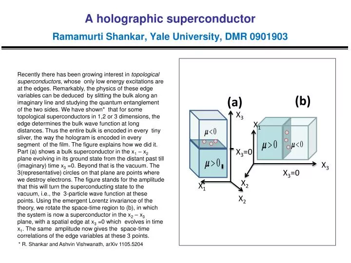
(b) (a) X3 X3=0 X1 X2 A holographic superconductorRamamurti Shankar, Yale University, DMR 0901903 Recently there has been growing interest in topological superconductors, whose only low energy excitations are at the edges. Remarkably, the physics of these edge variables can be deduced by slitting the bulk along an imaginary line and studying the quantum entanglement of the two sides. We have shown* that for some topological superconductors in 1,2 or 3 dimensions, the edge determines the bulk wave function at long distances. Thus the entire bulk is encoded in every tiny sliver, the way the hologram is encoded in every segment of the film. The figure explains how we did it. Part (a) shows a bulk superconductor in the x1 – x2 plane evolving in its ground state from the distant past till (imaginary) time x3 =0. Beyond that is the vacuum. The 3(representative) circles on that plane are points where we destroy electrons. The figure stands for the amplitude that this will turn the superconducting state to the vacuum, i.e., the 3-particle wave function at these points. Using the emergent Lorentz invariance of the theory, we rotate the space-time region to (b), in which the system is now a superconductor in the x2 – x3 plane, with a spatial edge at x3 =0 which evolves in time x1. The same amplitude now gives the space-time correlations of the edge variables at these 3 points. * R. Shankar and Ashvin Vishwanath, arXiv 1105.5204 X1 X3 X3=0 X2