Download

1 / 57
580 likes | 592 Views
Top down systems biology. Introduction systems biology 2011/2012 Huub Hoefsloot. Schedule. 09:00-09:45 lecture 09:45-11:00 coffee + assignments 1&2 11:00-11:45 lecture 11:45-12:45 coffee + assignment 3 13:30-15:15 MATLAB tutorials P323 15:15- ?? finish report F229

E N D
Top down systems biology Introduction systems biology 2011/2012 Huub Hoefsloot
Schedule • 09:00-09:45 lecture • 09:45-11:00 coffee + assignments 1&2 • 11:00-11:45 lecture • 11:45-12:45 coffee + assignment 3 • 13:30-15:15 MATLAB tutorials P323 • 15:15- ?? finish report F229 • 16:30-?? iGEM KC159
Aim • What is the top down approach? • Basic methods: • Clustering • Classification • Principal Component Analysis (PCA) • Looking at the single genes, proteins, metabolites, • How to draw biological conclusions?
Top down • Measure as much as possible • Let the data speak!!! • Common data types • Transcriptomics • Proteomics • Metabolomics
Methods • Clustering • Test single genes/proteins……. • Principal component analysis • Discrimination
Hierarchical clustering • Various hierarchical clustering algorithms exist • Single-linkage clustering, nearest-neighbor • Complete-linkage, furthest-neighbor • Average-linkage, un-weighted pair-group method average • Weighted-pair group average • ...
Hierarchical clustering • Small example 2 5 3 1 4
distances • Calculate the distances between all points • This yields n(n-1)/2 distances Y=pdist(X) 2.9155 1.0000 3.0414 3.0414 2.5495 3.3541 2.5000 2.0616 2.0616 1.0000 (1,2) (1,3) (1,4) (1,5) (2,3) (2,4) (2,5) (3,4) (3,5) (4,5)
Dendrogram (nearest) 2.9155 1.0000 3.0414 3.0414 2.5495 3.3541 2.5000 2.0616 2.0616 1.0000 (1,2) (1,3) (1,4) (1,5) (2,3) (2,4) (2,5) (3,4) (3,5) (4,5)
Furthest 2.9155 1.0000 3.0414 3.0414 2.5495 3.3541 2.5000 2.0616 2.0616 1.0000 (1,2) (1,3) (1,4) (1,5) (2,3) (2,4) (2,5) (3,4) (3,5) (4,5)
Clustering from a tree • Define a cut off value • Define a number of clusters.
An example http://www2.warwick.ac.uk/fac/sci/moac/students/peter_cock/r/heatmap/
Distances • Distances in Rn • Euclidean • City Block distance • Mahalanobis • . • . D is diagonal
: K-means clustering • The number of clusters has to be chosen in advance • Initial position of the cluster centers have to be chosen • For each data point the (euclidean, many more available) distance to each cluster center is calculated • Each data point is assigned to it‘s nearest cluster center • Cluster centers are shifted to the center of data points assigned to this cluster center • Step 3. – 5. is iterated until cluster centers are not shifted anymore
K-means Dividing line X X First guess for blues First guess for reds
K-means Dividing line X X Second guess for blues second guess for reds
K-means Dividing line X X Final result for blues Final result for reds
K-means • How to determine the number of clusters? • Try some and use a method to calculate the best.
What is the problem • 30000 genes are measured in a case control study • For each gene a t-test is performed at a significance level of α=0.05 • 1500 genes are found to be significant even if the two groups do not differ.
False positives/false negatives • False positives are variables that are found to differ but actually do not differ between the groups. • False negatives are variables that are not found by the test but actually do differ.
Bonferroni correction • If n tests are performed use adjusted values: αadj=α/n • This results in a procedure that the chance of finding a false negative in a set of n variables equals α.
Permutation approach • Permute the labels and make a nonsense data set. • Look for the number of significant variables many times. • The number of findings in the true data should be in the right tail of the distribution
Distribution found in permutations Only significant (with a level of 0.05) if the result is in the right hand side 5% of the permutation distribution Frequency The false discovery rate can be calculated using the mean of the permutation distribution 5% Number of genes found
Result is a list of genes • What to do with this list? • How to get a biological interpretation? • Look if the genes in the list are related. • See, with the help of GO if some biological processes are overrepresented. (Bioinformatics)
Assignment 1 • Read the primer on gene expression clustering. (ignore SOM) Answer the following question: • Come up with a biological question in which Pearson correlation and not an Euclidian distance. Please explain!
Assignment 2 • Read primer on multiple testing and answer the following question: • What is the advantages of an empirical null and what are the advantages of an analytical null?
Principal Components Analysis An intuitive explanation
Points in space x1 Object 1 Object 2 Object 3 Object 4 x1 0 1 2 3 4
Points in space x1 x2 Object 1 4 Object 2 3 Object 3 Object 4 2 1 x1 0 1 2 3 4
Points in space x1 x2 x3 x2 Object 1 4 x3 Object 2 3 Object 3 Object 4 2 1 x1 0 1 2 3 4 Objects are points in R3
Points in space x1 x2 x3 xn Object 1 ………… Object 2 Object 3 Object 4 Objects are points in Rn
How to visualize Rn? • Use 2 variables only? Many, many plots!! This does not help. • Find “important” directions. And plot the objects with respect to these directions. This is the idea behind Principal Component Analysis (PCA).
Important directions x2 x2 x1 x1 Covariance?
Principal components x2 PC1 PC2 x1
Any gain? Only consider the most important components PC1 projection PC1
Dimension reduction • From 2D to 1D is a small gain • From 30000D to 2D is a lot and a plot (visualization) can be made.
What are the results of a PCA loading score
= principal component Scores and loadings loadings ... + + DATA scores Scores tell something about an object Loadings about the variables
Explained variance • PCA tries to explain variance in the data • First PC explain as much variance as possible • The next PC explain as much as possible from the remainder
Question • In what group does an object belong
Discriminant analysis LDA Linear discriminant analysis PCDA Principal component discriminant analysis
Multivariate normal distribution No co-variance, equal variance
Linear discriminant analysis (LDA) D Discriminant direction m2 m1 Dividing line
Multivariate normal With covariance
Linear discriminant analysis (LDA) M2 Discriminant direction M1
LDA calculations W is the pooled within class covariance D is the discriminant vector