Download
1 / 30
310 likes | 336 Views
Geo Information Systems Part 5 Prof. Dr.-Ing. Raimar J. Scherer Institute of Construction Informatics Dresden, 05.07.2006. Metrical adjacency sizes. x. x. x. Distance between 2 areas. minimal. centre of gravity (Distance of centres). optional.

E N D
Geo Information SystemsPart 5 Prof. Dr.-Ing. Raimar J. SchererInstitute of Construction InformaticsDresden, 05.07.2006
Metrical adjacency sizes x x x Distance between 2 areas minimal centre of gravity (Distance of centres) optional Example of misleading distances: Epicentral Distance e.g. earthquake M=7 with approx. 70x20 km rupture plane strong earthquake damages occure in the radius of ca. 70 km Building x Epicentre 70 x 20 = 1.400 70² - p = 15.000 i.e.: about 10 % of all places would have distance d = 0 but their epicentral distance given is d ≤ 35 km all other distances are overestimated by up to 35 km or even up to 70 km if epicentre is at the border of the rupture plain. This lead to big errors in the PGA Peak Ground Acceleration attenuation laws: PGA = f(distance)
Shortest Way 2-step solution • compute the shortest distance between each 2 neighbouring vertices using the triple algorithm • search the shortest distance in number of edges and add all smallest distances of these edges The triple algorithmn computes all shortes ways in a weighted graph. It defines a matrix with all possible connections and assigns to each cell the sum of its ways. For a given problem this matrix can be computed in advance. It is a matrix with the dimension n² (n=number of nodes). After this, a way between two nodes can be read directly from the matrix. But this shows also the problem of this approach: Even if only one shortes way shall be determined, the algorithm needs to handle all node tripels. Furthermore the way table has to be stored, which especially in case of minor occupied adjacent matrices leads to enormous memory. From the combination of the way table with the incidence matrix results the shortest connections with the net.
Shortest Way, Triple-Algorithm Triple Algorithm (s. D. Jungnickel, 1987): The algorithm solves this problem in order O(|n|³), where n is the number of vertices Compute for each neighbouring vertices the shortest distance by evaluating all possible ways between the 2 vertices (i,j) with 1 additional vertix (k) and keep the shortes distance of the two possibilities, namely d(i,j) or [d(i,k)+d(k,j)]. Doing this for all possible i,j we end up in an iterative way with the shortest distance between each (i,j) For i = 1,n For j = 1,n For k = 1,n d(i,j) = min {d(i,j), d(i,k)+d(k,j)} i k j
Shortest Way, Example A 1(p=7) B 2(p=6) 3(p=1) E 6(p=2) 5(p=1) D C 7(p=5) For the given graph the shortest distance between each 2 vertices is sought. p = speed t = d/v, Sum time in [min]
Shortest Way, Example A 1(p=7) B 2(p=6) 3(p=1) E 6(p=2) 5(p=1) D C 7(p=5) Given graph Weighting matrix
Shortest Way, Example A 1(p=7) B 2(p=6) 3(p=1) E 6(p=2) 5(p=1) D C 7(p=5) Incidence matrix Adjacent matrix
Shortest Ways, Example Totals of Shortest Ways
Example for direct computing • Develope tree with support of adjacent matrix • Pick all pathes with leaves A • Compute distance Adjacent Matrix A M P A S T U A X Y . . . . . . . E . . . . F B . . . . G A C
Presentation Data-/ Information-/ Knowledge-Presentation = Visualisation through • geometrical graphic (mathematical exactly) • photorealistic graphic (human readable) • Symbolism (representation of non-visual facts) • diagrams • alphanumeric tables • reports
Object oriented data structure Object class Graph. Representation T1 Tn Thematic 0-C Point Line Polyline=face Geometric Topologie (prim) Object 3-C Volume Topologie 0-C Thematic Topologie (prim) 3-C Object ID Geometrie 2D 2D + 1D unlinked model 2,5 D point with height attr. 3D Vector 4 D Metric 2 D Point exact Primary Metric Raster 0D IDs Secondary Metric Names Addresses
Information acquisition Amount of data/information is very huge • exactness / resolution <-> efficiency • photogrammetry – surface model of site • visual interpretation of pictures is currently most often used – objects, meta-information • remote sensing – object identification, meta-information, attributes information of vegetation only semi-automatic supervised classification (lerned with testbeds) • other acquisition methods- data acquisition on site: measuring or counting- interviews- continous measurement acquisition (gaging station)- positioning- seismic methods- boring
Information retrieval Classification : 1 correlating value Intersection : 2 correlating values amax - distribution Topographyerection phase (=damage) intensity distribution Map of Los Angeles 1994 earthquake Map of Los Angeles 1994 earthquake intensity -> vector coast line -> grid city ?? -> grid calculated max a -> vector (circles)
Data Analysis Goal • identification of spatial interdependencies in one theme (statistic analysis) • identification of location based interdependencies between different themes • identification of spatial interdependencies between different themes • identification of interactions and resulting changes (=simulation)
Metric metric = distance function d(P,Q) Definition: d(P,Q) = 0 -> PºQ > 0 -> P¹Q = d(Q,P) =< d(P,R) + d(R,Q) possible metrics are: Euklid de ( å (pi – qi)²)1/2 (to long) City Block d4å (pi – qi) (to short) Chess board d8 max { |(pi – qi)| } the following relations can be given:
Correlation of Topics • Statistical methods • describing statistics • analytical statistics • Measurement scales • nominal scale : description (word, letter, number) • ordinal scale : hierarchy • (metric scales) • interval scale (without zero-point multiplikation not possible) • rational scale (with zero-point)
Correlation of Topics • Analytical statistics • univariate statistics : 1 variable • bivariate statistics : 2 variables • multivariate statistics : n variables
Correlation of themes It is easy, if there are location-related objects in each theme. It is the case for raster data. Remind, raster data have very little information content. z object class 1 object class 2 y object class 3 x
Overlay of Points and Areas + + + + + 1 7 4 + + 6 + + + 8 2 + + + + + + + + 3 5 Points – Object class 1 Area – Object class 1 2 1 + 8 objects 2 objects Overlay + Result – Object class 3 + 5 objects
Overlay of Curve and Area Curve – Object class 1 Area – Object class 1 1 2 3 3 2 1 4 3 objects 4 objects Overlay Result – Object class 3 1 3 2 4 6 5 6 objects
Overlay of Area and Area Area – Object class 1 Area – Object class 1 2 2 1 3 3 1 4 4 4 objects 4 objects Overlay Result – Object class 3 4 2 3 1 5 7 11 9 6 10 8 6 objects
Vertex in Area Test 3 2 1 vertex • rectangle inside if: y,xmin£ y,x £ y,xmax • polygon: test-ray: vertex – test-vertex, • test-vertex must be outside • if the number of cuts with polygon: • odd-numbered = inside • even = outside fast pre-test on outside with envelope rectangle (a) Test 2 1 Vertex
polygon cluster point cluster point cluster 70 90 80 100 90 110 70 80 90 100 110 isoline interpolation neighbourship graph zentroid determination
Statistical methods fundamental terms and coherences see lecture Prof. Herz measured values point estimator: mean value: modally value: median value: x = x50% I F(x) = 0,50 quantile value: xq = x I F(x) = q%
Statistical methods interval estimator: span with: D = xmax – xmin mean deviation: variance: deviation: variation coefficient:
Probability P(a<xb) = fx(x)dx = F(a) – F(b) P(a=x) = 0
Normal distribution standardised (i.e. σU=1, mU=0) due to symmetry it applies, that
Classification For the assignment (classification) of an object (area etc.) to a set it is required e.g. that min. X% of the objects' elements hold the characteristic properties. P(-s≤u≤s) = 68% P(-2s≤u≤2s) = 95.5% P(-3s≤u≤3s) = 97.7% 90 % ≙ P(u1.65s) 95 % ≙ P(u1. 96s) 99 % ≙ P(u2.58s) 99.5 % ≙ P(u3.29s)
Dependency between 2 variables(bivariate statistical methods) Mean value center Standard distance Correlation coefficient Covariance
Regression line(Fitting of a straight line) ? y x Condition: