Download
1 / 31
310 likes | 453 Views
Hash Tables. Hash Tables. Motivation: Dictionaries Set of key/value pairs We care about search, insertion, and deletion We typically don’t care about sorted order Example: given a student’s SSN, give their GPA. Hash Tables. More formally:

E N D
Hash Tables David Luebke 111/7/2014
Hash Tables • Motivation: Dictionaries • Set of key/value pairs • We care about search, insertion, and deletion • We typically don’t care about sorted order • Example: given a student’s SSN, give their GPA. David Luebke 211/7/2014
Hash Tables • More formally: • Given a table T and a record x, with key (= symbol) and satellite data, we need to support: • Insert (T, x) • Delete (T, x) • Search(T, x) • We want these to be fast, but don’t care about sorting the records • The structure we will use is a hash table • Supports all the above in O(1) expected time! David Luebke 311/7/2014
Hashing: Keys • In the following discussions we will consider all keys to be (possibly large) natural numbers • How can we convert ASCII strings to natural numbers for hashing purposes? David Luebke 411/7/2014
Direct Addressing • Suppose: • The range of keys is 0..m-1 • Keys are distinct • The idea: • Set up an array T[0..m-1] in which • T[i] = x if x T and key[x] = i • T[i] = NULL otherwise • This is called a direct-address table • Operations take O(1) time! • So what’s the problem? David Luebke 511/7/2014
The Problem With Direct Addressing • Direct addressing works well when the range m of keys is relatively small • But what if the keys are 32-bit integers? • Problem 1: direct-address table will have 232 entries, more than 4 billion • Problem 2: even if memory is not an issue, the time to initialize the elements to NULL may be • Solution: map keys to smaller range 0..m-1 • This mapping is called a hash function David Luebke 611/7/2014
Example: SSN’s • Suppose we have student records, that we want to index by the key of social security numbers. • Direct Addressing means having an array of 1,000,000,000 entries • What if I just have an array of 5,000,000 entries and divide each number by two before putting the record in the array? • Dividing by two is the hash function • What’s the problem with doing this? David Luebke 711/7/2014
Hash Functions • Next problem: collision T 0 U(universe of keys) h(k1) k1 h(k4) k4 K(actualkeys) k5 h(k2) = h(k5) k2 h(k3) k3 m - 1 David Luebke 811/7/2014
Resolving Collisions • How can we solve the problem of collisions? • Solution 1: chaining • Solution 2: open addressing David Luebke 911/7/2014
Open Addressing • Basic idea • To insert: if slot is full, try another slot, …, until an open slot is found (probing) • To search, follow same sequence of probes as would be used when inserting the element • If reach element with correct key, return it • If reach a NULL pointer, element is not in table • Good for fixed sets (adding but no deletion) David Luebke 1011/7/2014
Open Addressing Hashing • Approach • Hash table contains objects • Probe examine table entry • Collision • Move K entries past current location • Wrap around table if necessary • Find location for X Examine entry at A[ key(X) ] If entry = X, found If entry = empty, X not in hash table Else increment location by K, repeat David Luebke 1111/7/2014
Open Addressing Hashing • Approach • Linear probing • Move one slot in the table at a time • May form clusters of contiguous entries • Deletions – the tricky part • Find location for X • If X inside cluster, leave non-empty marker • Insertion • Find location for X • Insert if X not in hash table • Can insert X at first non-empty marker David Luebke 1211/7/2014
Open Addressing Example • Hash codes • H(A) = 6 H(C) = 6 • H(B) = 7 H(D) = 7 • Hash table • Size = 8 elements • = empty entry • * = non-empty marker • Linear probing • Collision move 1 entry past current location 12345678 David Luebke 1311/7/2014
Open Addressing Example • Operations (A=>6, B =>7, C=>6, D=>7) • Insert A, Insert B, Insert C, Insert D A 12345678 AB 12345678 ABC 12345678 DABC 12345678 David Luebke 1411/7/2014
Open Addressing Example • Operations (A=>6, B =>7, C=>6, D=>7) • Find A, Find B, Find C, Find D DABC 12345678 DABC 12345678 DABC 12345678 DABC 12345678 David Luebke 1511/7/2014
Open Addressing Example • Operations (A=>6, B =>7, C=>6, D=>7) • Delete A, Delete C, Find D, Insert C D*BC 12345678 D*B* 12345678 D*B* 12345678 DCB* 12345678 David Luebke 1611/7/2014
Types of Probing • Linear: If there’s a collision, skip by a constant number of entries (we did 1 at a time) • Problem: creates clusters • Quadratic probing: for k, the key, and i, the number of times I’ve probed so far, h(k,i) = (h’(k) + ci + di2) mod m where c and d are constants and h’ is yet another hash function • Result: the more collisions I get, the more space I skip David Luebke 1711/7/2014
Types of Probing • Double hashing h(k,i) = (h1(k) + i*h2(k)) mod m for h1 and h2 auxiliary hash functions. • first hash depends on h1 only • collisions skip different amounts • Some of the best hash functions in practice are double hash functions David Luebke 1811/7/2014
Chaining • Chaining puts elements that hash to the same slot in a linked list: T —— U(universe of keys) k1 k4 —— —— k1 —— k4 K(actualkeys) k5 —— k7 k5 k2 k7 —— —— k3 k2 k3 —— k8 k6 k8 k6 —— —— David Luebke 1911/7/2014
Chaining • How do we insert an element? T —— U(universe of keys) k1 k4 —— —— k1 —— k4 K(actualkeys) k5 —— k7 k5 k2 k7 —— —— k3 k2 k3 —— k8 k6 k8 k6 —— —— David Luebke 2011/7/2014
Chaining • How do we delete an element? T —— U(universe of keys) k1 k4 —— —— k1 —— k4 K(actualkeys) k5 —— k7 k5 k2 k7 —— —— k3 k2 k3 —— k8 k6 k8 k6 —— —— David Luebke 2111/7/2014
Chaining • How do we search for a element with a given key? T —— U(universe of keys) k1 k4 —— —— k1 —— k4 K(actualkeys) k5 —— k7 k5 k2 k7 —— —— k3 k2 k3 —— k8 k6 k8 k6 —— —— David Luebke 2211/7/2014
Analysis of Chaining • Assume simple uniform hashing: each key in table is equally likely to be hashed to any slot • Given n keys and m slots in the table: the load factor = n/m = average # keys per slot • What will be the average cost of an unsuccessful search for a key? David Luebke 2311/7/2014
Analysis of Chaining • Assume simple uniform hashing: each key in table is equally likely to be hashed to any slot • Given n keys and m slots in the table, the load factor = n/m = average # keys per slot • What will be the average cost of an unsuccessful search for a key? A: O(1+) David Luebke 2411/7/2014
Analysis of Chaining • Assume simple uniform hashing: each key in table is equally likely to be hashed to any slot • Given n keys and m slots in the table, the load factor = n/m = average # keys per slot • What will be the average cost of an unsuccessful search for a key? A: O(1+) • What will be the average cost of a successful search? David Luebke 2511/7/2014
Analysis of Chaining • Assume simple uniform hashing: each key in table is equally likely to be hashed to any slot • Given n keys and m slots in the table, the load factor = n/m = average # keys per slot • What will be the average cost of an unsuccessful search for a key? A: O(1+) • What will be the average cost of a successful search? A: O(1 +/2) = O(1 + ) David Luebke 2611/7/2014
Analysis of Chaining Continued • So the cost of searching = O(1 + ) • If the number of keys (n) is proportional to the number of slots in the table (m), what is ? • A: = O(1) • In other words, we can make the expected cost of searching constant if we make constant David Luebke 2711/7/2014
Choosing A Hash Function • Clearly choosing the hash function well is crucial • What will a worst-case hash function do? • What will be the time to search in this case? • What are desirable features of the hash function? • Should distribute keys uniformly into slots • Should not depend on patterns in the data David Luebke 2811/7/2014
Hash Functions: Worst Case Scenario • Scenario: • You are given an assignment to implement hashing • You will self-grade in pairs, testing and grading your partner’s implementation • In a blatant violation of the honor code, your partner: • Analyzes your hash function • Picks a sequence of “worst-case” keys, causing your implementation to take O(n) time to search • What’s an honest CS student to do? David Luebke 2911/7/2014
Hash Functions: Universal Hashing • As before, when attempting to foil an malicious adversary: randomize the algorithm • Universal hashing: pick a hash function randomly in a way that is independent of the keys that are actually going to be stored • Guarantees good performance on average, no matter what keys adversary chooses David Luebke 3011/7/2014
Practice • 11.2-2 Demonstrate the insertion of the following keys into a hash table with collisions resolved by chaining. Let the table have 9 slots and let the hash function be h(k) = k mod 9. • Keys are: 5,28,19,15,20,33,12,17,10 • Do the same for an open address table with linear probing. David Luebke 3111/7/2014