Download

1 / 48
490 likes | 614 Views
Desirability Indexes for Soft Constraint Modeling in Drug Design. Johannes Kruisselbrink E-mail: jkruisse@liacs.nl. Scope. Context: Quality measures for candidate molecular structures for automated optimization Contents:

E N D
Desirability Indexes for Soft Constraint Modeling in Drug Design Johannes Kruisselbrink E-mail: jkruisse@liacs.nl
Scope Context: • Quality measures for candidate molecular structures for automated optimization Contents: • Using the concept of Desirability for modeling soft or fuzzy constraints • The applicability in automated drug design and examples for integration within a scoring function
f1max / min f2max / min | fmmax / min G O A L S Objectives System (Model) Output Y Input X g1 ≤ 0 g2 ≤ 0 | gn ≤ 0 Constraints External (uncontrollable) parameters A Uncertainty and noise in optimization problems Uncertainty and noise can arise in various parts of the optimization model: C) Uncertain and/or noisy system output A) Uncertainty and noise in the design variables B) Uncertainty and noise environmental parameters D) Vagueness / fuzziness in the constraints
Automated molecule design • Search for molecular structures with specific pharmacological or biological activity • Objectives: Maximization of potency of drug (and minimization of side-effects) • Constraints: Stability, synthesizability, drug-likeness, etc. • Aim: provide a set of molecular structures that can be promising candidates for further research
Initialize population P0 While not terminate do Generate offspring O from P Pt+1= select from (P U O) Evaluate O Molecule Evolution ‘Normal’ evolution cycle Graph based mutation and recombination operators Deterministic elitist (μ+λ) parent selection (NSGA-II with Niching) Fragments extracted from From Drug Databases “The molecule evoluator. An interactive evolutionary algorithm for the design of drug-like molecules.“, E.-W. Lameijer, J.N. Kok, T. Bäck, A.P. IJzerman, J. Chem. Inf. Model., 2006, 46(2): 545-552.
Objectives and constraints Objectives • Activity predictors based on support vector machines: • f1: activity predictor based on ECFP6 fingerprints • f2: activity predictor based on AlogP2 Estate Counts • f3: activity predictor based on MDL Constraints • Bounds based on Lipinski’s rule of five and the minimal energy confirmation: • Number of Hydrogen acceptors • Number of Hydrogen donors • Molecular solubility • Molecular weight • AlogP value • Minimized energy
Soft constraints in Drug Design • Estimating the feasibility of candidate structures can be done using boundary values for certain molecule properties • Examples are Lipinski’s rule-of-five and estimations of the minimal energy conformations • But…, how strict are those rules? • Sometimes violations are easy to fix manually • Sometimes violations are not violations in practice
Molecules failing Lipinski log P (5.088) MW log P MW Atorvastatin Ethopropazine Bexarotene Liothyronine HA / HD MW / HA MW / HA Doxycycline Olmesartan Acarbose
The real nature of the constraints The constraints are of the following forms: Where • x denotes a candidate structure • g(x) denotes the property value of x • Aj is the lower bound of the property filter • Bj is the upper bound of the property filter • reads: A is preferred to be smaller than B
Modeling constraints as objectives Constraints can be transformed into ‘objectives’ by mapping their values onto a function with the domain <0,1> where: • Values close to 0 correspond to undesirable results • Values close to 1 correspond to desirable results • Values between 0 and 1 fall into the grey area Cutoff bound 1 1 Constraint bound 0 0 Two-sided One-sided violated grey area satisfied violated grey area satisfied grey area violated There are multiple ways to create such mappings!
Constraints in our studies Fuzzy constraint scores based on Lipinski’s rule of five and bounds on the minimal energy confirmation: * Bounds settings were determined based on chemical intuition
One-sided: Two-sided: Harrington Desirability Functions
Example one-sided Harrington DF Molecular solubility: • Soft constraint: Y > -4 • Absolute cutoff: Y < -6 violated grey area satisfied
Example two-sided Harrington DF Molecular weight: • Absolute lower cutoff: Y < 150 • Lower bound constraint: Y > 250 • Upper bound constraint: Y < 450 • Absolute upper cutoff: Y > 600 Problematic! • No support for non-symmetric boundaries • No explicit support for ‘completely satisfied’ intervals
grey area violated grey area violated satisfied Example two-sided Harrington DF One possibility: • Make symmetric • Base d(Y) on cutoff bounds • Tune n using a constraint bound
grey area violated grey area violated satisfied Example two-sided Harrington DF Or: • Make symmetric • Base d(Y) on constraint bounds • Tune n using a cutoff bound
Example two-sided Harrington DF Or: Make symmetric Base d(Y) on average between constraint bounds and cutoff bounds Tune n using a cutoff bound grey area violated grey area violated satisfied
Harrington • Advantages: • Maps onto a continuous function • Strictly monotonous mapping • Distinction between completely violated points • Downsides: • Tuning the DF is somewhat arbitrary • Distinction between completely satisfied solutions • Not really suited for ‘completely satisfied intervals’ • Does not allow non-symmetric constraints
One-sided: Two-sided: Derringer Desirability Functions
violated grey area satisfied Example one-sided Derringer DF Molecular solubility: • Soft constraint: Y > -4 • Absolute cutoff: Y < -6 Note: l=1linear
grey area violated grey area violated satisfied Example two-sided Derringer DF Molecular weight: • Absolute cutoff: Y < 150 • Soft constraint: Y > 250 • Soft constraint: Y < 450 • Absolute cutoff: Y > 600
Derringer • Advantages: • Easy straightforward implementation • Control for modeling non-symmetric constraints • Easy integration for ‘completely satisfied’ intervals • No distinction between completely satisfied solutions • Downsides: • Maps onto a discontinuous function • Not strictly monotonous (just monotonous) • No distinction between solutions after lower cutoff
Many objective optimization • Modeling fuzzy constraints using DFs generates many additional objective functions • In our case: • 3 original objectives + 6 constraints 9 objectives • The possibilities: • Pareto optimization • Aggregation • A combination of the both
Aggregation • Desirability functions can be easily integrated into one single scoring function, e.g.: • Weighted sum • Min performance • Geometrical mean • Average The Desirability Index
Remodeling the objectives • Desirability index aggregation of the objectives requires a normalization function that maps the objective function values to the interval [0,1] • One possibility: • Or…, use Harrington or Derringer DFs Original objective function minimization
The aggregation possibilities • Full aggregation: • Aggregate the constraints and the objectives into one quality score (1 objective) • Partial aggregation: • Aggregate the constraints into one constraint score (1 extra objective 4 objectives) • Aggregate the constraints and the objectives into two separate scoring function (2 objectives)
Experiments Comparison of: • Complete aggregation (1 objective) • Separate aggregation of objectives and constraints (2 objectives) • Only aggregate constraint scores (4 objectives) Objectives: • three activity prediction models for estrogen receptor antagonists EA settings: • NSGA-II for the multi-objective test-cases • 80 parents / 120 offspring • 1000 generations • No niching
4D Pareto fronts Optimization direction Only aggregate constraint scores (4 objectives) Complete aggregation (1 objective) The Pareto fronts obtained using three different scoring methods Aggregate constraints and objectives separately (2 objectives)
Separate constraints and objectives Tamoxifen Color: constraint scores (white = 0 black = 1) f3: MDL max (=1) f2: ECFP max (=1) f1: AlogP2 EC max (=1)
1 0 grey area satisfied violated Discussion - Ranking issues • DFs that can yield 0 values will generate 0 values for the performance when aggregating using the geometric mean • DFs that make distinctions between completely satisfied constraints might be involved in unnecessary further optimization (maximization while already satisfied) An ideal DF? Never 0 (distinction on the degree of constraint) When satisfied 1 (no distinction between satisfied regions)
Conclusions • Desirability Functions and Desirability Indexes for modeling soft / fuzzy constraints: • Are intuitive and easy to incorporate • Allow for easy integration of additional constraints • Incorporate the concept of vagueness present in all rule-of-thumb measures • Prevent the optimization method from ruling out promising candate structures
Thank you! Johannes Kruisselbrink Natural Computing Group LIACS, Universiteit Leiden e-mail: jkruisse@liacs.nl http://natcomp.liacs.nl
Matlab codes(no presentation stuff, just for creating the DF plots)
Harrington one-sided example clf x = [0:.1:10]; y = exp(-exp(-(-8 + 2 * x))); plot(x, y) ylim([-.1 1.1]) xlabel('Y') ylabel('d(Y)')
Harrington two-sided example clf x = [0:.01:10]; y = exp(-abs((2 * x - (6 + 4))/(6 - 4)).^(3)); plot(x, y) ylim([-.1 1.1]) xlabel('Y') ylabel('d(Y)')
One-sided Harrington DF in MATLAB clf x = [-8:.1:-2]; y = exp(-exp(-(16.8548 + 3.0637 * x))); plot(x, y) hold on plot([-8 -6 -4 -2],[0 0 1 1], '-.r') ylim([-.1 1.1]) xlabel('Y') ylabel('d(Y)') legend('Harrington DF', 'Linear DF', 'Location', 'NorthWest')
Two-sided Harrington DF 1 in MATLAB clf x = [0:1:800]; y = exp(-abs((2 * x - (600 + 150))/(600 - 150)).^(7.8273)); plot(x, y) hold on plot([0 150 250 450 600 850], [0 0 1 1 0 0], '-.r') ylim([-.1 1.1]) xlabel('Y') ylabel('d(Y)') legend('Harrington DF', 'Linear DF', 'Location', 'NorthEast')
Two-sided Harrington DF 2 in MATLAB clf x = [0:1:800]; y = exp(-abs((2 * x - (450 + 250))/(450 - 250)).^(2.2033)); plot(x, y) hold on plot([0 150 250 450 600 850], [0 0 1 1 0 0], '-.r') ylim([-.1 1.1]) xlabel('Y') ylabel('d(Y)') legend('Harrington DF', 'Linear DF', 'Location', 'NorthEast')
Two-sided Harrington DF 3 in MATLAB clf x = [0:1:800]; y = exp(-abs((2 * x - (525 + 200))/(525 - 200)).^(5.6927)); plot(x, y) hold on plot([0 150 250 450 600 850], [0 0 1 1 0 0], '-.r') ylim([-.1 1.1]) xlabel('Y') ylabel('d(Y)') legend('Harrington DF', 'Linear DF', 'Location', 'NorthEast')
One-sided Derringer DF in MATLAB clf hold on x = [-8:.01:-2]; y1 = (x >= -4) * 1 + (x < -4) .* (x >= -6) .* ((x + 6)/(-4 + 6)).^0.5; plot(x, y1, '-.b') y2 = (x >= -4) * 1 + (x < -4) .* (x >= -6) .* ((x + 6)/(-4 + 6)).^1; plot(x, y2, '--r') y3 = (x >= -4) * 1 + (x < -4) .* (x >= -6) .* ((x + 6)/(-4 + 6)).^2; plot(x, y3, 'g') ylim([-.1 1.1]) xlabel('Y') ylabel('d(Y)') legend('Derringer DF (l=0.5)', 'Derringer DF (l=1)', 'Derringer DF (l=2)', 'Location', 'NorthWest')
Two-sided Derringer DF in MATLAB clf hold on x = [0:.1:800]; y1 = (x >= 150) .* (x < 250) .* ((x - 150) / (250 - 150)).^(0.5) + (x >= 250) .* (x <= 450) .* 1 + (x > 450) .* (x <= 600) .* ((x - 600) / (450 - 600)).^(0.5); plot(x, y1, '-.b') y2 = (x >= 150) .* (x < 250) .* ((x - 150) / (250 - 150)).^(1) + (x >= 250) .* (x <= 450) .* 1 + (x > 450) .* (x <= 600) .* ((x - 600) / (450 - 600)).^(1); plot(x, y2, '--r') y3 = (x >= 150) .* (x < 250) .* ((x - 150) / (250 - 150)).^(2) + (x >= 250) .* (x <= 450) .* 1 + (x > 450) .* (x <= 600) .* ((x - 600) / (450 - 600)).^(2); plot(x, y3, 'g') ylim([-.1 1.1]) xlabel('Y') ylabel('d(Y)') legend('Derringer DF (l=0.5)', 'Derringer DF (l=1)', 'Derringer DF (l=2)', 'Location', 'NorthEast')