Download
1 / 38
390 likes | 399 Views
272: Software Engineering Fall 2008. Instructor: Tevfik Bultan Lecture 16: Dynamic Invariant Discovery. Specifications. We saw various specification techniques contracts for classes JML object oriented design OCL, Alloy interfaces Interface grammars, interface state machines

E N D
272: Software Engineering Fall 2008 Instructor: Tevfik Bultan Lecture 16: Dynamic Invariant Discovery
Specifications • We saw various specification techniques • contracts for classes • JML • object oriented design • OCL, Alloy • interfaces • Interface grammars, interface state machines • All these specification techniques help software developers to document the design decisions at a higher level of abstraction than the code
Specifications • There is one problem with software specifications • Software developers do not like to write them! • I personally believe that it is all about cost/benefit ratio • If there is enough benefit in writing specifications • reduced development time, more reliable programs, etc. • then people will write specifications • Maybe current tools and techniques used in software development do not provide enough benefit for writing specifications • This may change in the future based on all the techniques and tools we discussed in this course
Lack of Specifications • However, the fact remains, there is a lot of code out there with no specifications • maybe even no comments • What should we do about them? • You may say “Why do I care? I write detailed specifications when I develop software.” • There may be some code written by somebody else that you need to maintain, modify, or reuse • none of the original developers may still be around • there may not be any specifications • the specifications may not have been maintained with the software
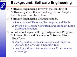
Reverse Engineering • Reverse engineering is the process of analyzing a subject system • to identify the system’s components and their inter-relationships, and • to create representations of the system in another form or at a higher level of abstraction • Examples • Producing call graphs or control flow graphs from the source code • Generating class diagrams from the source code • Two types of reverse engineering • Redocumentation: the creation or revision of a semantically equivalent representation within the same relative abstraction layer • Design recovery: involves identifying meaningful higher level abstractions beyond those obtained directly by examining the system itself
Reverse Engineering • The main goal is to help with the program comprehension • Most of the time reverse engineering makes up for lack of good documentation • We already saw a reverse engineering technique (a design recovery technique): • Automated interface extraction
Dynamically Discovering Likely Invariants • Today I will talk about another reverse engineering approach • References • ``Dynamically discovering likely program invariants to support program evolution,’’ Michael D. Ernst, Jake Cockrell, William G. Griswold, and David Notkin. IEEE Transactions on Software Engineering, vol. 27, no. 2, Feb. 2001, pp. 1-25. • ``Quickly detecting relevant program invariants,’’ Michael D. Ernst, Adam Czeisler, William G. Griswold, and David Notkin. ICSE 2000, Proceedings of the 22nd International Conference on Software Engineering, pp. 449-458. • There is also a tool which implements the techniques described in the above papers • Daikon • works on C, C++, Java, Lisp
Dynamically Discovering Likely Invariants • The main idea is to discover likely program invariants from a given program • In this work, an ``invariant’’ means an assertion that holds at a particular program point (not necessarily all program points) • They discover likely program invariants • there is no guarantee that the discovered invariants will hold for all executions
Dynamically Discovering Likely Invariants • Discovered properties are not stated in any part of the program • They are discovered by monitoring the execution of the program on a set of inputs (a test set) • The only thing that is guaranteed is that the discovered properties hold for all the inputs in the test set • No guarantee of soundness or completeness
An Example • An example from “The Science of Programming,” by Gries, 1981 • A good references on programming using assertions, Hoare Logic, weakest preconditions, etc. Program 15.1.1 // Sum array b of length n into variable s i = 0; s = 0; while (i != n) { s = s + b[i]; i = i+1; } • Precondition: n 0 • Postcondition: s = ( j : 0 j n : b[j]) • Loop invariant: 0 i n and s = ( j : 0 j i : b[j])
An Example • The test set used to discover invariants has 100 randomly-generated arrays • Length is uniformly distributed from 7 to 13 • Elements are uniformly distributed from –100 to 100 • Daikon discovers invariants by • running the program on this test set • monitoring the values of the variables
Discovered Invariants Size of the test set 15.1.1:::ENTER 100 samples N = size(B) (7 values) N in [7..13] (7 values) B (100 values) All elements >= -100 (200 values) • These are the assertions that hold at the entry to the procedure • likely preconditions • The invariant in the box implies the precondition of the original program (it is a stronger condition that implies the precondition that N is non-negative) Number of distinct values for N
Discovered Invariants 15.1.1:::EXIT 100 samples N = I = orig(N) = size(B) (7 values) B = orig(B) (100 values) S = sum(B) (96 values) N in [7..13] (7 values) B (100 values) All elements >= -100 (200 values) • These are the assertions that hold at the procedure exit • likely postconditions • Note that orig(B) corresponds to Old.B in contracts
Discovered Invariants 15.1.1:::LOOP 1107 samples N = size(B) (7 vallues) S = sum(B[0..I-1]) (452 values) N in [7..13] (7 values) I in [0..13] (14 values) I <= N (77 values) B (100 values) All elements in [-100..100] (200 values) sum(B) in [-556..539] (96 values) B[0] nonzero in [-99..96] (79 values) B[-1] in [-88..99] (80 values) B[0..I-1] (985 values) All elements in [-100..100] (200 values) N != B[-1] (99 values) B[0] != B[-1] (100 values) • These are the assertions that hold at the loop entry and exit • likely loop invariants Means last element
A Different Test Set • Instead of using a uniform distribution for the length and the contents of the array an exponential distribution is used • The expected values for the array lengths and the element values are same for both test sets
Discovered Invariants 15.1.1:::ENTER 100 samples N = size(B) (24 values) N >= 0 (24 values)
Discovered Invariants 15.1.1:::EXIT 100 samples N = I = orig(N) = size(B) (24 vallues) B = orig(B) (96 values) S = sum(B) (95 values) N >= 0 (24 values)
Discovered Invariants 15.1.1:::LOOP 1107 samples N = size(B) (24 vallues) S = sum(B[0..I-1]) (858 values) N in [0..35] (24 values) I >= 0 (36 values) I <= N (363 values) B (96 values) All elements in [-6005..7680] (784 values) sum(B) in [-15006..21244] (95 values) B[0..I-1] (887 values) All elements in [-6005..7680] (784 values)
Dynamic Invariant Detection • How does dynamic invariant generation work? • Run the program on a test set • Monitor the program execution • Look for potential properties that hold for all the executions
Dynamic Invariant Detection • Instrument the program to write data trace files • Run the program on a test set • Offline invariant engine reads data trace files, checks for a collection of potential invariants Data traces Instrument Run Detect Invariants Original Program Invariants Test set
Inferring Invariants • There are two issues • Choosing which invariants to infer • Inferring the invariants • Daikon infers invariants at specific program points • procedure entries • procedure exits • loop heads (optional) • Daikon can only infer certain types of invariants • it has a library of invariant patterns • it can only infer invariants which match to these patterns
Trace Values • Daikon supports two forms of data values • Scalar • number, character, boolean • Sequence of scalars • All trace values must be converted to one of these forms • For example, an array A of tree nodes each with left and a right child would be converted into two arrays • A.left (containing the object IDs for the left children) • A.right
Invariant Patterns • Invariants over any variable x (where a, b, c are computed constants) • Constant value: x = a • Uninitialized: x = uninit • Small value set: x {a, b, c} • variable takes a small set of values • Invariants over a single numeric variable: • Range limits: x a, x b, a x b • Nonzero: x 0 • Modulus: x = a (mod b) • Nonmodulus: x a (mod b) • reported only if x mod b takes on every value other than a
Invariant Patterns • Invariants over two numeric variables x, y • Linear relationship: y = ax + b • Ordering comparison: x y, x y, x y, x y, x = y, x y • Functions: y = fn(x) or x = fn(y) • where fn is absolute value, negation, bitwise complement • Invariants over x+y • invariants over single numeric variable where x+y is substituted for the variable • Invariants over x-y
Invariant Patterns • Invariants over three numeric variables • Linear relationship: z = ax + by + c, y=ax+bz+c, x=ay+bz+c • Functions z = fn(x,y) • where fn is min, max, multiplication, and, or, greatest common divisor, comparison, exponentiation, floating point rounding, division, modulus, left and right shifts • All permutations of x, y, z are tested (three permutations for symmetric functions, 6 permutations for asymmetric functions)
Invariant Patterns • Invariants over a single sequence variable • Range: minimum and maximum sequence values (based on lexicographic ordering) • Element ordering: nondecreasing, nonincreasing, equal • Invariants over all sequence elements: such as each value in an array being nonnegative
Invariant Patterns • Invariants over two sequence variables: x, y • Linear relationship: y = ax + b, elementwise • Comparison: x y, x y, x y, x y, x = y, x y (based on lexicographic ordering) • Subsequence relationship: x is a subsequence of y • Reversal: x is the reverse of y • Invariants over a sequence x and a numeric variable y • Membership: x y
Inferring Invariants • For each invariant pattern • determine the constants in the pattern • stop checking the invariants that are falsified • For example, • For invariant pattern x a we have to determine the constant a • For invariant pattern x = ay + bz + c we have to determine the constants a, b, c
Inferring Invariants • Consider the invariant pattern: x = ay + bz + c • Consider an example data trace for variables (x, y, z) (0,1,-7), (10,2,1), (10,1,3), (0, 0,-5), (3, 1, -4), (7, 1, 1), ... • Based on the first three values for x, y, z in the trace we can figure out the constants a, b, and c 0 = a -7b +c 10 = 2a + b +c 10 = a +3b + c If you solve these equations for a, b, c you get: a=2, b=1, c=5 • The next two tuples (0, 0,-5), (3, 1, -4) confirm the invariant • However the last trace value (7, 1, 1) kills this invariant • Hence, it is not checked for the remaining trace values and it is not reported as an invariant
Inferring Invariants • Determining the constants for invariants are not too expensive • For example three linearly independent data values are sufficient for figuring out the constants in the pattern x = ay + bz + c • there are at most three constants in each invariant pattern • Once the constants for the invariants are determined, checking that an invariant holds for each data value is not expensive • Just evaluate the expression and check for equality
Cost of Inferring Invariants • The cost of inferring invariants increases as follows: • quadratic in the number of variables at a program point (linear in the number of invariants checked/discovered) • linear in the number of samples or values (test set size) • linear in the the number of program points • Typically a few minutes per procedure: • 10,000 calls, 70 variables, instrument entry and exit
Invariant Confidence • Not all unfalsified invariants should be reported • There may be a lot of irrelevant invariants which may just reflect properties of the test set • If a lot of spurious invariants are reported the output may become unreadable • Improving (increasing) the test set would reduce the number of spurious invariants
Invariant Confidence • For each detected invariant Daikon computes the probability that such a property would appear by chance in a random input • If that probability is smaller than a user specified confidence parameter, then the property is reported • Daikon assumes a distribution and performs a statistical test • It checks the probability that the observed values for the detected invariant were generated by chance from the distribution • If that probability is very low, then the invariant is reported
Invariant Confidence • As an example, consider an integer variable x which takes values between r/2 and -r/2-1 • Assume that x0 for all test cases • If the values of x is uniformly distributed between r/2 and -r/2-1, then the probability that x is not 0 is 1 – 1/r • Given s samples the probability x is never 0 is (1-1/r)s • If this probability is less than a user defined confidence level then x0 is reported as an invariant
Derived Variables • Looking for invariants only on variables declared in the program may not be sufficient to detect all interesting invariants • Daikon adds certain derived variables (which are actually expressions) and also detects invariants on these derived variables
Derived Variables • Derived from any sequence s: • Length: size(s) • Extremal elements: s[0], s[1], s[size(s)-1], s[size(s)-2] • Daikon uses s[-1] to denote s[size(s)-1] and s[-2] to denote s[size(s)-2] • Derived from any numeric sequence s: • Sum: sum(s) • Minimum element: min(s) • Maximum element: max(s)
Derived Variables • Derived from any sequence s and any numeric variable i • Element at the index: s[i], s[i-1] • Subsequences: s[0..i], s[0..i-1] • Derived from function invocations: • Number of calls so far
Dynamically Detecting Invariants: Summary • Useful reengineering tool • Redocumentation • Can be used as a coverage criterion during testing • Are all the values in a range covered by the test set? • Can be helpful in detecting bugs • Found bugs in an existing program in a case study • Can be useful in maintaining invariants • Prevents introducing bugs, programmers are less likely to break existing invariants