Download
1 / 34
340 likes | 344 Views
A Methodology for automatic retrieval of similarly shaped machinable components. Mark Ascher - Dept of ECE. Motivation. Retrieval of similarly shaped components can: Add functionality to existing CAD databases

E N D
A Methodology for automatic retrieval of similarly shaped machinable components Mark Ascher - Dept of ECE
Motivation • Retrieval of similarly shaped components can: • Add functionality to existing CAD databases • allow for the reuse of process plans which can both speed up and reduce the cost of development. Challenges • Retrieval of similarly shaped components has many challenges: • Multiple interpretations • Interacting features • Topological differences do not guarantee component dissimilarity • Graph matching solution is computationally intensive
Contributions • Retrieval of sub pieces to cover a component • Use of Maximal Feature Sub-graphs to divide a component • Use of type abstraction hierarchies to guide similarity search • Feature and interaction Histogram based • Ability to abstract Features and Interactions of machinable components • Ability to determine distances of features and interactions based on objective criterion
Related Work • Shape Based Similarity Retrieval (Eakins) • Two dimensional parts • retrieved complete components • Volumetric Reasoning (Lee et al) and Planar Reasoning (Cohn et al) • Groundwork for symbolic volumetric reasoning • Does not address part matching • Content Retrieval From Images Based on Knowledge of Shape (Hsu et al) • Worked with medical images • Presented the Type Abstraction Hierarchy Concept
Related Work • 3D Model Shape Based Similarity Retrieval (Osada et al, Regli et al) • Uses D2 Distance measures • Works well for simple models • Feature Based Model Retrieval (Regli et al) • Retrieves complete models • Feature interaction representation too simplistic • No method for indexing
Related Work • Group Technology • Goal is to group components by similar machining processes for improved factory flow • Similar machining processes does not guarantee shape similarity
Query Evaluator System Overview User Interface Query In B-Rep Query Answer Feature Extractor Spatial Logic Spatial Logic Geometric Modeler Query Relaxation Component Database Block Handler
Component Representation In the Database • Data Represented in Three Layers • Raw B-Rep Component (Representation Layer) • Graph of Maximal Features and Interactions (Knowledge Layer) • Histograms of Features and Abstracted Interactions (Semantic Layer) • Interactions Encoded at Multiple Abstraction Levels • Interaction Matrix • Set of Face Pairs • Abstracted Interaction
R5,2 Interactions • Interactions Represented as an nxm matrix where: • n is the number of faces in feature 1(f1) • m is the number of faces in feature 2 (f2) • Entries are in the set { +, -, s, i} • + indicates that f1 lies in the positive half space of f2 • - indicates that f1 lies in the negative half space of f2 • s indicates they lie on the same plane • I indicates that the features interact
Interactions Continued • If only orthonormal features are considered • Results in 6x6 interaction Matrices • The near diagonal data points contain the pertinent data • The number of unique columns is reduced to 5 ordered types that are physically valid • The following notation indicates (same, opposite) face • (-,+) No Interaction • (-,s) indicates a shared face with no internally shared points • (-,-) indicates a face that is interior to both faces of the other feature • (s,-) indicates a shared face with internally shared points • (+,-) indicates a face that is not interior to one face of the other feature • The following Combinations are invalid: • (+,+) can not be outside both faces parallel to the face of interest • (s,s) can not be the same as two faces which bound a feature • (+,s) and (s,+) can not be same as one face and outside the other
(s, -) (-,-) 2 1 Interactions Continued (+,-) (-,s) (+,-) -1 0 3
Interactions Continued • Pairs of parallel Faces are compared Resulting in 7 Feasible Unordered face-pair Combinations: Type Face 1 Face 2 Relation of faces to other Feature D (s,-) (s,-) Both Faces Shared B (s,-) (-,-) One Face Shared Other Inside (+,-) E (s,-) One face shared, Other Outside Opp (s,-) (-,s) Not Possible A (-,-) (-,-) Both Faces Inside C (-,-) (+,-) One Face Inside, Other Outside (-,-) (-,s) Not Possible F (+,-) (+,-) Both Outside G (+,-) (-,s) One Face Shared, Other Outside (-,s) (-,s) Not Possible
Type Face 1 Face 2 Inverse Interaction D (s,-) (s,-) D B (s,-) (-,-) E (+,-) E (s,-) B A (-,-) (-,-) F C (-,-) (+,-) C F (+,-) (+,-) A G (+,-) (-,s) G Interactions Continued • Inverse Relations Exist for some Face-pair Types. B D A E F C G
Interactions Continued • Several Face-pair types indicate a family of interactions. Type Face 1 Face 2 Interaction Family E -s -+ Intrusion C -- -+ Improper Interaction F -+ -+ Pass Through G -+ +s Face
Interactions Continued Each Interaction can be represented by three Face-pairs
Spatial Logic Spatial Logic Query Evaluator System Overview User Interface Query In B-Rep Query Answer Feature Extractor Geometric Modeler Query Relaxation Component Database Block Handler
Spatial Logic • The Spatial Logic Utilizes Knowledge encoded in the interactions to: • Reduce Computations to determine Interactions • Determine Closest Matches from Candidate Pool • Guide Query Relaxation • Invalidate Non-Maximal Features • Spatial Logic Applied in One Dimension • 3D Accomplished by combining 1D results • 3D Uses Facts About Maximal Features to: • Reduce Number of Reasoned Interactions • Guide Quantitative Interaction Determination
Second Interaction P1 to P3 First Interaction P1 to P2 Inferred Interaction P2 to P3 Face Pair F Logic (1,1) Face Pair A Logic (3,3) Face Pair A Logic (1,1) One Dimensional Examples • New Face Pair Completely Determined • Qualitative Interaction in this dimension known • No Quantitative Computation Required
Second Interaction P1 to P3 First Interaction P1 to P2 Inferred Interaction P2 to P3 Face Pair F Logic (1,3) Face Pair A Logic (3,3) Face Pair A,B,C Logic (1,y) One Dimensional Examples • New Face Pair Incompletely Determined • One face determinable • Quantitative Computation Required for One Face
One Dimensional Examples First Interaction P1 to P2 Second Interaction P1 to P3 Inferred Interaction P2 to P3 Face Pair C, G None Logic (3,z) Face Pair F Logic (1,3) Face Pair F Logic (3,1) • New Face Pair Incompletely Determined • One face determinable • Interaction Existence In-determinable • Quantitative Computation Required for One Face
One Dimensional Examples First Interaction P1 to P2 Second Interaction P1 to P3 Inferred Interaction P2 to P3 Face Pair Undeterminable Logic (U) Face Pair F Logic (1,1) Face Pair F Logic (1,1) • New Face Pair Undeterminable • Not enough information to make any determination • Existence of an interaction unknown • Quantitative Computation Required for both Faces
Value 3 11 12 13 21 22 23 30 31 32 33 3 2y N 30 3y N 30 3y N N 30 3y 11 N U x3 x3 3x 33 33 N 3x 33 33 12 3 yz y2 y3 3z 32 33 N 3z 32 33 13 1y yz y1 yy 3z 31 3y N 3z 31 3y 21 N zy z3 z3 2y 23 23 30 3y 33 33 22 3 11 12 13 21 22 23 30 31 32 33 23 1y 11 11 1y 21 21 2y 30 31 31 3y 30 N N N N 3 3 3 y2 y3 y3 y3 31 N zy z3 z3 1y 13 13 y1 yy y3 y3 x – -1,0,1,2,3, y – 1,2,3, z – -1,0,1, N – no interaction, U - unknown 32 3 11 12 13 11 12 13 y1 y1 y2 y3 33 1y 11 11 1y 11 11 1y y1 y1 y1 yy Inferencing Table
Spatial Logic Continued • Maximal Features Reduce the Possible Results • No maximal feature can be subsumed by any other single feature • No maximal feature can have an entire face end in the interior of another feature. • No maximal feature shall subsume any other maximal feature • Intersecting Maximal feature must share at least one point interior to a face
Example Logic Application 3 Dimensions Interaction 2 II-2 B, E, C [(2,1), (3,2) (3,1)] Interaction 1 PI-2a B,E,B [(2,1), (2,3), (2,1)] (2,y) (3,1) (3,y) Implies Improper
Logic Experiments • Interactions presented as the set of interactions were encoded as drawn (no rotations) • The interactions were selected pair-wise as submission to the Spatial-Logic • The following data was collected • Number of physically possible interaction • Number of interactions possible for Maximal Features
Experimental Results • 23 Interactions Compared (529 total pairs) • 84 Completely Determined – 15.9% (78 No Interaction) • 55 1 undetermined face – 10.4% • 94 2 undetermined faces – 17.8% • 124 3 undetermined faces – 23.4% • 103 4 undetermined faces – 19.5% • 60 5 undetermined faces – 11.3% • 9 No faces determined 1.7% • Maximal Feature Constraints Reduced The Number Of Possibilities an Additional 33.9%
Query Evaluator System Overview User Interface Query In B-Rep Query Answer Feature Extractor Spatial Logic Spatial Logic Geometric Modeler Query Relaxation Component Database Block Handler
Example Database • An example database was generated to test out the process • Features were encoded as histograms of feature types • Features used were Slots, Blind Slots, Steps, Blind Steps, and Pockets • No other feature information was encoded • Only maximal features were encoded • Interactions were encoded as histograms of interaction types present (I.e. PI-0, PI-1, etc.) • Two levels of abstraction were used for features and interactions • Feature abstractions used the following abstraction scheme: • distinct features • combine blind and through of each type • combine all slots and steps • Interaction abstractions used the following abstraction scheme: • Distinct interactions • Combine all proper or improper interactions of individual types • Combine all interactions of individual types (pass-through, intrusion, etc)
Example Database • Each Component was encoded along with any sub-parts. • Each Component and Sub-part was then submitted to the database to find the closest match • Distances were calculated as the vector distance between the feature histogram plus the vector distance between the interaction histogram • For abstraction the histogram entries were reduced based on the abstraction scheme • Results for all combinations of feature and interaction abstraction levels were determined • Features and interactions were equally weighted
Example Database Selected Results • Component 1 returned matches of components 10 and 25 • Sub part 1 returned component 10 • Sub part 2 returned components 11 and 25 • Component 9 returned component 8 and both sub-parts from 7 • Component 7 returned component 16 but sub parts returned component 8 • Component 17 returned component 32 • Component 28 returned components 20 and 23 • Component 25 returned components 11, 20 and 26
Example Database Results Summary • Generally reasonable results were achieved • The returned parts were qualitatively what would be expected • Spatial Logic Not Utilized • Matching would be improved • Interaction Type Lowest Level of Knowledge Encoded
Future Work • Generate Database of More Complex Parts • Implement Spatial Logic with Database • Query Evaluation Unit • Spatial Logic Symbology