Download
1 / 16
170 likes | 178 Views
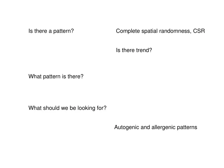
Is there a pattern?. Complete spatial randomness, CSR. Is there trend?. What pattern is there?. What should we be looking for?. Autogenic and allergenic patterns. Watt 1947. Analysis of Spatial Dependence.

E N D
Is there a pattern? Complete spatial randomness, CSR Is there trend? What pattern is there? What should we be looking for? Autogenic and allergenic patterns
Analysis of Spatial Dependence Traditional methods are based on data types that have origins (sometimes multiple) in different subjects Point data distance statistics ( ) Point data with values variogram Gridded data spatial autocorrelation near neighbours Moran statistic etc all neighbours 2-D autocorrelation & spectral analysis Are we dealing with: transformations of the data estimating parameters of a model and does it matter?
Example of point at the Crane Site Abies amabilis Pseudotsuga Taxus brevifolia Thuja plicata Tsuga heterophylla y Data collected by: Freeman (1997) Ishii et al. (2000) x (meters)
A: area of plot i :subject tree dij j :other trees dij :distance between i and j t t : radius of circle It (dij) : indicator function wij : weighting factor, correct for edge effects L(t) = K(t) / π-t Transform K to L; K(t)
G(t) :Nearest Neighbor L(t) : All pairs of Trees L12(t) All Inter-type Pairs Cumulative frequency distributions
L(t): All pairs of Trees G(t): Nearest Neighbor Clumped Clumped Clumped Clumped
regular regular L(t) for increasingly restricted Height Classes 13+m Height Class
Acer circinatum Abies amabilis Taxus brevifolia Thuja plicata Tsuga heterophylla Seedling Regeneration Maps Clumped Overstory Regular Overstory 32m square in Subplot 8 32m square in Subplot 13 y (meters) x(meters) x(meters)
The problem of simultaneous inference Simulation envelop for the G (nearest neighbor statistic built from 99 simulations for λ=100 on a unit square. Solid line indicates simulation envelope limits. Red ‘o’ marks where a transition to a different pattern comprising that section of the limit. In this example 63 of the 99 simulated patterns contribute to the envelope at some distance. The probability that a CSR pattern would exceed the displayed envelope is 63/99 ~ 0.63 much higher than the normal error rate. Loosmore & Ford 2006
Calculation of a single summary statistic for each realization and the data tmax tk is distance Ui = [ Hi(tk) – Hi(tk)]2 tk _ tmin and tmax are the lower and upper distance limits > tk = tmin Hi (tk) is the empirical result for pattern i for the test statistic of interest (G or K), Hi (tk) is the mean result computed for all patterns except for i tk= (tk+1 – tk) is the width of the distance interval Parameter estimation for a simple clumping model using ui based on the G and K statistics
Point data with values – the variogram Read Western et al. 1998
Two dimensional autocorrelation and spectral analysis For method and illustration read: Renshaw and Ford (1984) For application read: Johan van de Koppel, and Caitlin Mullan Crain (2006)