Download

1 / 97
970 likes | 994 Views
Explore query processing steps, SQL to relational algebra translation, sorting algorithms, and heuristics for optimization in database systems.

E N D
Query Processing and Optimization Outline (Ch. 18, 3rd – Ch. 15, 4th ed. 5th ed., Ch. 19, 6th ed., Ch. 18, 19, 7th ed.) • Processing a high-level query • Translating SQL queries into relational algebra • Basic algorithms • Sorting: internal sorting and external sorting • Implementing the SELECT operation • Implementing the JOIN operation • Implementing the Project operation • Other operations • Heuristics for query optimization Dr. Yangjun Chen ACS-4902
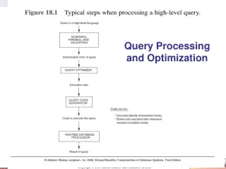
Steps of processing a high-level query Query in a high-level language Scanning, Parsing, Validating Query code generation Intermediate form of query Code to execute the query Query optimization Runtime database processor Execution plan Result of query Dr. Yangjun Chen ACS-4902
Translating SQL queries into relational algebra - decompose an SQL query into query blocks query block - SELECT-FROM-WHERE clause Example: SELECT LNAME, FNAME FROM EMPLOYEE WHERE SALARY > (SELECT MAX(SALARY) FROM EMPLOEE WHERE DNO = 5); SELECT MAX(SALARY) FROM EMPLOYEE WHERE DNO = 5 SELECT LNAME, FNAME FROM EMPLOYEE WHERE SALARY > c inner block outer block Dr. Yangjun Chen ACS-4902
Translating SQL queries into relational algebra - translate query blocks into relational algebra expressions SELECT MAX(SALARY) FROM EMPLOYEE WHERE DNO = 5 F MAX SALARY(DNO=5(EMPLOYEE)) SELECT LNAME, FNAME FROM EMPLOYEE WHERE SALARY > c LNAME FNAME(SALARY>C(EMPLOYEE)) Dr. Yangjun Chen ACS-4902
Basic algorithms - sorting: internal sorting and external sorting - algorithm for SELECT operation - algorithm for JOIN operation - algorithm for PROJECT operation - algorithm for SET operations - implementing AGGREGATE operation - implementing OUTER JOIN Dr. Yangjun Chen ACS-4902
Basic algorithms - internal sorting - sorting in main memory: sort a series of integers, sort a series of keys sort a series of records - different sorting methods: simple sorting merge sorting quick sorting heap sorting Dr. Yangjun Chen ACS-4902
Basic algorithms - different internal sorting methods: sorting numbers Input n numbers. Sort them such that the numbers are ordered increasingly. 3 9 1 6 5 4 8 2 10 7 1 2 3 4 5 9 7 8 9 10 Dr. Yangjun Chen ACS-4902
Basic algorithms - A simple sorting algorithm main idea: 1st step: 3 9 1 6 5 4 8 2 10 7 2nd step: 1 9 3 6 5 4 8 2 10 7 1 2 3 6 5 4 8 9 10 7 … ... swap swap Dr. Yangjun Chen ACS-4902
Basic algorithms - A simple sorting algorithm Algorithm Input: an array A containing n integers. Output: sorted array. 1. i := 2; 2. Find the least element a from A(i) to A(n); 3. If a is less than A(i - 1), exchange A(i - 1) and a; 4. i := i + 1; goto step (2). Time complexity: O(n2) Dr. Yangjun Chen ACS-4902
Heapsort • What is a heap? • MaxHeap and Maintenance of MaxHeaps - MaxHeapify - BuildMaxHeap • Heapsort - Algorithm - Heapsort analysis Dr. Yangjun Chen ACS-4902
Heapsort • Combines the better attributes of merge sort and insertion sort. • Like merge sort, but unlike insertion sort, running time is O(n lg n). • Like insertion sort, but unlike merge sort, sorts in place. • Introduces an algorithm design technique • Create data structure (heap) to manage information during the execution of an algorithm. • The heap has other applications beside sorting. • Priority Queues Dr. Yangjun Chen ACS-4902
Data Structure Binary Heap • Array viewed as a nearly complete binary tree. • Physically – linear array. • Logically – binary tree, filled on all levels (except lowest.) • Map from array elements to tree nodes and vice versa • Root – A[1], Left[Root] – A[2], Right[Root] – A[3] • Left[i] – A[2i] • Right[i] – A[2i+1] • Parent[i] – A[i/2] A[2] A[3] A[i] A[2i] A[2i + 1] Dr. Yangjun Chen ACS-4902
24 21 23 22 36 29 30 34 28 27 21 23 36 29 30 22 34 28 Data Structure Binary Heap • length[A] – number of elements in array A. • heap-size[A] – number of elements in heap stored in A. • heap-size[A] length[A] 24 1 1 2 3 4 5 6 7 8 9 10 2 3 Searching the tree in breadth-first fashion, we will get the array. 4 5 6 7 27 8 9 10 Dr. Yangjun Chen ACS-4902
Heap Property (Max and Min) • Max-Heap • For every node excluding the root, the value stored in that node is at most that of its parent: A[parent[i]] A[i] • Largest element is stored at the root. • In any subtree, no values are larger than the value stored at the subtree’s root. • Min-Heap • For every node excluding the root, the value stored in that node is at least that of its parent: A[parent[i]] A[i] • Smallest element is stored at the root. • In any subtree, no values are smaller than the value stored at the subtree’s root Dr. Yangjun Chen ACS-4902
26 24 20 18 17 19 13 12 14 11 24 20 17 19 13 18 12 14 Heaps – Example Max-heap as an array. 1 2 3 4 5 6 7 8 9 10 Max-heap as a binary tree. 26 1 2 3 4 5 6 7 11 Last row filled from left to right. 8 9 10 Dr. Yangjun Chen ACS-4902
Heaps in Sorting • Use max-heaps for sorting. • The array representation of a max-heap is not sorted. • Steps in sorting (i) Convert the given array of size n to a max-heap (BuildMaxHeap) (ii) Swap the first and last elements of the array. • Now, the largest element is in the last position – where it belongs. • That leaves n – 1 elements to be placed in their appropriate locations. • However, the array of first n – 1 elements is no longer a max-heap. • Float the element at the root down one of its subtrees so that the array remains a max-heap (MaxHeapify) • Repeat step (ii) until the array is sorted. Dr. Yangjun Chen ACS-4902
Heap Characteristics • Height = lg n • No. of leaves = n/2 • No. of nodes of height h n/2h+1 . . . height(aleaf) = 0 n/22+1 n/21+1 n/20+1 Dr. Yangjun Chen ACS-4902
Maintaining the heap property • Suppose two subtrees are max-heaps, but the root violates the max-heap property. • Fix the offending node by exchanging the value at the node with the larger of the values at its children. • May lead to the subtree at the child not being a max heap. • Recursively fix the children until all of them satisfy the max-heap property. Dr. Yangjun Chen ACS-4902
MaxHeapify –Example MaxHeapify(A, 2) 1 26 26 2 3 24 24 18 24 14 20 14 20 14 14 4 5 6 7 17 17 19 19 18 24 14 14 24 18 18 14 14 24 13 13 9 10 8 12 12 14 18 14 18 11 11 Dr. Yangjun Chen ACS-4902
Procedure MaxHeapify MaxHeapify(A, i) 1. l left(i) (* A[l] is the left child of A[i] .*) 2. r right(i) 3. ifl heap-size[A] and A[l] > A[i] 4. thenlargest l 5. elselargest i 6.ifr heap-size[A] andA[r] > A[largest] 7. thenlargest r 8. if largest i • then exchange A[i] A[largest] • MaxHeapify(A, largest) Assumption: Left(i) and Right(i) are max-heaps. A[largest] must be the largest among A[i], A[l] and A[r]. Dr. Yangjun Chen ACS-4902
Running Time for MaxHeapify • MaxHeapify(A, i) • 1. l left(i) • 2. r right(i) • 3. ifl heap-size[A] and A[l] > A[i] • 4. thenlargest l • 5. elselargest i • 6.ifr heap-size[A] andA[r] > A[largest] • 7. thenlargest r • 8. if largest i • 9. then exchange A[i] A[largest] • 10. MaxHeapify(A, largest) Time to fix node i and its children = (1) PLUS Time to fix the subtree rooted at one of i’s children = T(size of subree at largest) Dr. Yangjun Chen ACS-4902
Running Time for MaxHeapify(A, n) • T(n)= T(size of subree at largest) + (1) • size of subree at largest 2n/3 (worst case occurs when the last row of tree is exactly half full) • T(n) T(2n/3) + (1) T(n)= O(lg n) • Alternately, MaxHeapify takes O(h)where h is the height of the node where MaxHeapify is applied Dr. Yangjun Chen ACS-4902
Building a Max-heap • Use MaxHeapify to convert an array A into a max-heap. • How? • Call MaxHeapify on each element in a bottom-up manner. BuildMaxHeap(A) 1. heap-size[A] length[A] 2. forilength[A]/2downto 1 (*A[length[A]/2 +1], 3. doMaxHeapify(A, i) A[length[A]/2 +2], … are leaf nodes.*) Dr. Yangjun Chen ACS-4902
24 21 23 22 36 29 30 34 28 27 21 23 36 29 30 22 34 28 BuildMaxHeap – Example Input Array: Initial Heap: (notmax-heap) 24 1 2 3 4 5 6 7 27 8 9 10 Dr. Yangjun Chen ACS-4902
BuildMaxHeap – Example MaxHeapify(10/2 = 5) MaxHeapify(4) 1 24 36 24 MaxHeapify(3) MaxHeapify(2) 21 30 34 24 21 23 36 23 3 2 MaxHeapify(1) 36 36 27 29 36 21 30 23 28 34 22 24 22 4 5 6 7 34 22 24 28 27 21 9 8 10 Dr. Yangjun Chen ACS-4902
Heapsort • Sort by maintaining the as yet unsorted elements as a max-heap. • Start by building a max-heap on all elements in A. • Call BuildMaxHeap(A) • Maximum element is in the root, A[1]. • Move the maximum element to its correct final position. • Exchange A[1] with A[n]. • Discard A[n] – it is now sorted. • Decrement heap-size[A]. • Restore the max-heap property on A[1..n–1]. • Call MaxHeapify(A, 1). • Repeat until heap-size[A] is reduced to 2. Dr. Yangjun Chen ACS-4902
Heapsort(A) • HeapSort(A) • 1. BuildMaxHeap(A) • 2. forilength[A] downto 2 • 3. do exchange A[1] A[i] • 4. heap-size[A] heap-size[A] – 1 • 5. MaxHeapify(A, 1) Time complexity: O(n·logn) Dr. Yangjun Chen ACS-4902
26 17 20 18 24 19 13 12 14 11 26 17 24 20 20 17 19 13 18 12 14 11 Heapsort – Example 1 2 3 4 5 6 7 8 9 10 26 Build-Max-heap 24 19 13 18 12 14 11 Dr. Yangjun Chen ACS-4902
24 24 18 17 19 13 12 13 11 18 11 14 17 19 11 12 14 14 11 26 18 17 11 13 12 12 19 11 24 18 17 19 13 14 20 26 Maxheapify 20 24, 26 Maxheapify 20 20 Dr. Yangjun Chen ACS-4902
18 12 14 12 18 11 12 11 14 18 17 13 17 11 17 12 18 12 12 14 11 17 14 20 13 20, 24, 26 Maxheapify 19 19 19, 20, 24, 26 19 Maxheapify 13 13 Dr. Yangjun Chen ACS-4902
17 11 14 12 12 14 12 11 11 14 14 12 11 12 11 17 18, 19, 20, 24, 26 18 Maxheapify 13 13 17, 18, 19, 20, 24, 26 17 Maxheapify 13 13 Dr. Yangjun Chen ACS-4902
12 12 11 12 11 11 11 12 14, 17, 18, 19, 20, 24, 26 14 Maxheapify 13 13 13, 14, 17, 18,19, 20, 24, 26 13 Maxheapify 11 11 Dr. Yangjun Chen ACS-4902
11 11 11 11 12, 13, 14, 17, 18, 19, 20, 24, 26 12 Maxheapify 11, 12, 13, 14, 17, 18,19, 20, 24, 26 11 Dr. Yangjun Chen ACS-4902
Algorithm Analysis HeapSort(A) 1. Build-Max-Heap(A) 2. forilength[A] downto 2 3. do exchange A[1] A[i] 4. heap-size[A] heap-size[A] – 1 5. MaxHeapify(A, 1) • In-place • BuildMaxHeap takes O(n)and each of the n-1 calls to MaxHeapify takes time O(lg n). • Therefore, T(n) = O(n lg n) Dr. Yangjun Chen ACS-4902
Basic algorithms - Sorting by merging Merging means the combination of two or more ordered sequence into a single sequence. For example, can merge two sequences: 503, 703, 765 and 087, 512, 677 to obtain a sequence: 087, 503, 512, 677, 703, 765. A simple way to accomplish this is to compare the two smallest items, output the smallest, and then repeat the same process. 503 703 765 087 512 677 503 703 765 512 677 087 703 765 512 677 087 503 Dr. Yangjun Chen ACS-4902
Basic algorithms - Merging algorithm Algorithm Merge(s1, s2) Input: two sequences: s1 - x1 x2 ... xm and s2 - y1 y2 ... yn Output: a sorted sequence: z1 z2 ... zm+n. 1.[initialize] i := 1, j := 1, k := 1; 2.[find smaller] if xi yjgoto step 3, otherwise goto step 5; 3.[output xi] zk.:= xi, k := k+1, i := i+1. If i m, goto step 2; 4.[transmit yj ... yn] zk, ..., zm+n := yj, ..., yn. Terminate the algorithm; 5.[output yj] zk.:= yj, k := k+1, j := j+1. If j n, goto step 2; 6.[transmit xi ... xm] zk, ..., zm+n := xi, ..., xm. Terminate the algorithm; Dr. Yangjun Chen ACS-4902
Basic algorithms - Merge-sorting Algorithm Merge-sorting(s) Input: a sequences s = < x1, ..., xm> Output: a sorted sequence. 1. If |s| = 1, then return s; 2. k := m/2; 3. s1 := Merge-sorting(x1, ..., xk); 4. s2 := Merge-sorting(xk+1, ..., xm); 5. return(Merge(s1, s2)); Dr. Yangjun Chen ACS-4902
center • Basic algorithms - quick sorting Pivot is 5. It will be stored in a temporary variable. main idea: 1st step: 3 1 6 5 4 8 10 7 2nd step: 3 2 1 5 8 9 10 7 3rd step: 3 2 1 4 5 6 8 9 10 7 from to 9 2 j i 6 4 i = j = 5 greater than 5 Smaller than 5 Dr. Yangjun Chen ACS-4902
center center • Basic algorithms - quick sorting from to 4th step: 4 5 6 10 5th step: 1 2 3 4 from to 2 8 1 9 7 3 i = 2 j = 2 Dr. Yangjun Chen ACS-4902
6th step: 1 The sequence contains only one element, no sorting. from to center The center element is 3. 7th step: 3 4 i = j = 1 8th step: 4 The sequence contains only one element, no sorting. 1 2 3 4 5 Dr. Yangjun Chen ACS-4902
6 8 9 10 7 6 7 8 9 10 Dr. Yangjun Chen ACS-4902
Basic algorithms - quick sorting main idea: Algorithm quick_sort(from, center, to) Input: from - pointer to the starting position of array A center - pointer to the middle position of array A to - pointer to the end position of array A Output: sorted array: A’ 0. i := from; j := to; if i = j, return; 1. Find the first element a = A(i) larger than or equal to A(center) from A(from) to A(to); (i is used to scan from left to right.) 2. Find the first element b = A(j) smaller than or equal to A(center) from A(to) to A(from); (j is used to scan from right to left.) 3. If i < j then exchange a and b; 4. Repeat step from 1 to 3 until j i; 5. If from < j then recursive call quick_sort(from,(from + j)/2, j); 6. If i < to then recursive call quick_sort(i, (i+ to)/2, to); Dr. Yangjun Chen ACS-4902
Basic algorithms - quick sorting Pivot is 18. 17, 2, 1, 14, 13, 12, 11, 8, 16, 15 3, 4, 6, 1, 10, 9, 5, 20, 19, 18, j i 17, 2, 1, 14, 13, 12, 11, 8, 16, 20 18, 19, 3, 4, 6, 1, 10, 9, 5, 15, 19, 20 3, 4, 6, 1, 10, 9, 5, 15, 16, 18, 17, 2, 1, 14, 13, 12, 11, 8, 18, 8, 17, 2, 1, 14, 13, 12, 11, 19, 20 3, 4, 6, 1, 10, 9, 5, 15, 16, i = 17 8, 17, 2, 1, 14, 13, 12, 11 3, 4, 6, 1, 10, 9, 5, 15, 16, j < i j = 16 Dr. Yangjun Chen ACS-4902
Basic algorithms - External sorting method: Sort records in a large file stored on disk that does not fit entirely in main memory. sort-merge sorting: 1. Divide the file into small files - called runs; 2. Sort phase: Sort runs in the buffer space in main memory; 3. Merge phase: Merge the sorted runs in turn. Dr. Yangjun Chen ACS-4902
Basic algorithms - External sorting method: Several parameters: b - number of file blocks nR - number of initial runs nB - available buffer space nR = b/ nB Example: nB = 5 blocks, b = 80 blocks, nR = 16 initial runs dM - number of runs that can be merged together in each pass Dr. Yangjun Chen ACS-4902
Basic algorithms - External sorting method: set i 1; j b; /*size of the file in blocks*/ k nB; /*size of buffer in blocks*/ m j/k; /*number of runs*/ /*sort phase*/ while (i m) do { read next k blocks of the file into the buffer or if there are less than k blocks remaining then read in the remaining blocks; sort the records in the buffer and write as a temporary subfile; i i +1; } Dr. Yangjun Chen ACS-4902
Basic algorithms - External sorting method: /*merge phase: merge subfiles until only 1 remains*/ set i 1; p logk-1 m; /*p is the number of passes for the merging phase*/ j m; /*number of runs*/ while (i p) do { n 1; q j /(k-1); /*q is the number of subfiles to write in this pass*/ while (n q) do { read next k-1 subfiles or remaining subfiles (from previous pass) one block at a time; merge and write as new subfile; n n + 1;} j q; i i + 1;} Dr. Yangjun Chen ACS-4902
4 5 7 18 20 21 8 10 19 30 40 51 6 9 12 13 15 17 • Example File contains 4 runs. 5 7 4 20 18 21 10 19 30 40 51 8 6 9 17 13 12 15 11 16 Buffer: 11 16 sorting phase Dr. Yangjun Chen ACS-4902
4 5 7 18 20 21 8 10 19 30 40 51 6 9 12 13 15 17 • Example temporary-file1: 4 5 … Buffer: 4 5 8 10 8 10 4 5 merging phase 11 16 Dr. Yangjun Chen ACS-4902
4 5 7 18 20 21 8 10 19 30 40 51 6 9 12 13 15 17 • Example temporary-file1: 4 5 7 8 … Buffer: 7 18 8 10 18 10 7 8 merging phase 11 16 Dr. Yangjun Chen ACS-4902