Download
1 / 46
460 likes | 463 Views
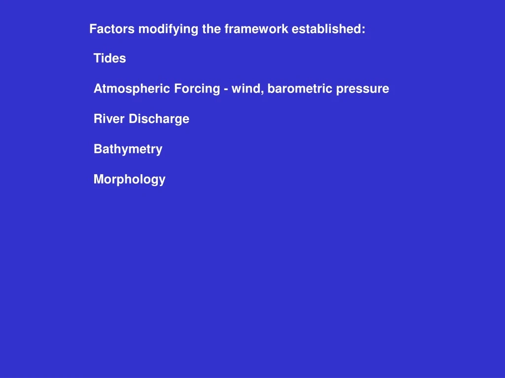
Factors modifying the framework established:. Tides Atmospheric Forcing - wind, barometric pressure River Discharge Bathymetry Morphology. TIDES. Tide - generic term to define alternating rise and fall in sea level with respect to

E N D
Factors modifying the framework established: Tides Atmospheric Forcing - wind, barometric pressure River Discharge Bathymetry Morphology
TIDES Tide - generic term to define alternating rise and fall in sea level with respect to land and is produced by the balance between the gravitational force (of the moon and sun mainly) and the centrifugal acceleration. Tide also occurs in large lakes, in the atmosphere, and within the solid crust Gravitational Force (Newton’s Law of Gravitation): F = GmM/R2 G = 6.67×10⁻¹¹ N m2/kg2
EQUILIBRIUM TIDE Centrifugal Force F = GmM/R2 Moon’s Gravitational Force (changes from one side of the earth to the other) Tide Generating Force (Difference between centrifugal and gravitational) Center of mass of Earth-Moon system ~1,700 km from Earth’s surface (because Earth is 81 times heavier than Moon) – Centrifugal = Gravitational
How strong is the Tide-Generating Force? Gravitational Force at A: B S A P Centrifugal Force at A: Imbalance (Tide-generating force at A): Tide-generating Force at A: Tide-generating Force at B:
How strong is the Tide-Generating Force? B S A P Tide-generating Force at A: Tide-generating Force at B: The mass of the sun is 2x1027 metric tons while that of the moon is only 7.3x10¹⁹ metric tons. The sun is 390 times farther away from the earth than is the moon. The relative Tide Generating Force on Earth = [(2x1027/7.3x1019)]/(3903) or = 2.7x10⁷/5.9x107 = 0.46 or 46%
Image from Hubble Telescope Equatorial Tides
Image from Hubble Telescope Tropic Tides
What alters the range and phase of tides produced by Equilibrium Theory? Non-astronomical factors: coastline configuration bathymetry atmospheric forcing (wind velocity and barometric pressure) hydrography may alter speed, produce resonance effects and seiching, storm surges In the open ocean, tidally induced variations of sea level are a few cm. When the tidal wave moves to the continental shelf and into confining channels, the variations may become greater.
Keep in mind that tidal waves travel as shallow (long) waves How so? Typical wavelengths = 4500 km (semidiurnal wave traveling over 1000 m of water) Ratio of depth / wavelength = 1 / 4500 C = [ gH ]0.5 Then, their phase speed is: The tide observed at any location is the superposition of several constituents that arise from diverse tidal forcing mechanisms. Main constituents:
The Form factor F = [ K1 + O1 ] / [ M2 + S2 ] is customarily used to characterize the tide. When 0.25 < F < 1.25 the tide is mixed - mainly semidiurnal When 1.25 < F < 3.00 the tide is mixed - mainly diurnal F > 3 the tide is diurnal F < 0.25 the tide is semidiurnal
When 0.25 < F < 1.25 the tide is mixed - mainly semidiurnal When 1.25 < F < 3.00 the tide is mixed - mainly diurnal F > 3 the tide is diurnal F < 0.25 the tide is semidiurnal Superposition of constituents generates modulation - e.g. fortnightly, monthly This applies for both sea level and velocity
In Ponce de León Inlet: M2 = 0.41 m; N2 = 0.09 m; O1: 0.06 m; S2: 0.06 m; K1= 0.08 m F = [K1 + 01] / [S2 + M2 ] = 0.30 GNV
Panama City In Panama City, FL: M2 = 0.085 m; N2 = 0.017 m; O1: 0.442 m; S2: 0.035 m; K1= 0.461 m F = [K1 + 01] / [S2 + M2 ] = 7.52
Co-oscillation Independent tide - caused by gravitational and centrifugal forces directly on the waters of the estuary -- usually small for typical dimensions of estuaries Co-oscillating tide - caused by the ocean tide at the entrance to the estuary as driving force The wave propagates into the basin and may be subject to RESONANCE and RECTIFICATION -- alters tidal flows and produces subtidal motions Let’s study what happens to the wave as it propagates into the estuary...
a time linear, partial differential equation (hyperbolic) The solution is d’Alembert’s solution, which can be studied with the sinusoidal wave form: Progressive wave Assume linear, frictionless motion in the x direction only, under homogeneous conditions. The momentum balance is then: And the continuity equation is:
a time a C/H time This indicates that the flow is in phase with the elevation
Standing wave And the continuity equation is: The solution is: The momentum balance is also:
a time time a C/H This indicates that the flow is out of phase with the elevation by 90 degrees
Resonance At the mouth x = L, L at x = L Substituting into and The natural period of oscillation is then: For resonance to exist, the denominator should tend to zero, i.e.,
u L Example of seiching For an estuary with length < λ /4, u is zero at the head and maximum at the mouth For longer estuaries u is zero at x = 0, λ / 2, 3 λ / 2,… or where sin κx = 0 and maximum at x = λ /4, 3 λ / 4, 5 λ / 4, …, i.e., where sin κx is max
Merion’s Formula Mode 1 (n =1)
Tidal Waves With Friction Integrating vertically: The bottom stressbecomes: Expanding this in a Fourier cosine series, to lowest order: With continuity: Momentum balance for a progressive wave: These are the governing equations for progressive tidal motion with friction.
and If we let We obtain the solution: where maximum U precedes maximum eta
Effects of Friction on a Standing Tidal Wave in an Estuary For resonance, we have again U =0 at the head of the estuary, i.e.,
Solution: Effects of Rotation on a Progressive Tidal Wave in a Semi-enclosed basin R = C / f KELVIN WAVE
Effects of Rotation on a Standing Tidal Wave in an Estuary Two Kelvin waves of equal amplitude progressing in opposite directions. Instead of having lines of no motion, we are now reduced to a central region -- amphidromic region-- of no motion at the origin. The interference of two geostrophically controlled simple harmonic waves produces a change from a linear standing wave to a rotary wave.
Effects of Bottom Friction on an amphydromic system Parker (1990)
Virtual Amphidromes Parker (1990)
Virtual amphidromes in Chesapeake Bay Fisher (1986)
Tidal Rectification Oscillatory tidal currents can produce a mean current or residual Noticeable in areas of sharp coastline bends and bathymetric gradients Non-linear phenomenon Energy is transferred from the dominant tidal frequencies (e.g. M2) to both higher harmonics (e.g. M4 and M6) and to mean flows (zero frequency). Three mechanisms responsible for this energy transfer to mean flow. Studied from vorticity tendencies.
Lateral Variations of Bottom Stress Lateral Shear in the Depth-Distributed Friction Force Conservation of Potential Vorticity Robinson (1981)
Tidal flow oscillations at a single frequency (e.g. M2) will generate tidal vorticity by the above 3 mechanisms. Taking the curl of that equation and which may be rewritten as: Because of non-linearities (products of u times u), the vorticity generated will not only be at the fundamental tidal frequency, but also at higher harmonics and at zero frequency. The three mechanisms can be identified from the vorticity equation. This is derived from the depth-averaged 2-D momentum equation appropriate to barotropic tidal motion in shallow seas
Max ebb End ebb Max flood End flood Example: Geyer and Signell (1990, JGR, 95, 3189)