Download
1 / 19
190 likes | 315 Views
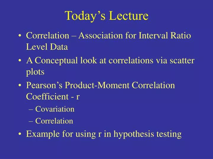
Today’s Lecture. Correlation – Association for Interval Ratio Level Data A Conceptual look at correlations via scatter plots Pearson’s Product-Moment Correlation Coefficient - r Covariation Correlation Example for using r in hypothesis testing. Reference Material.

E N D
Today’s Lecture • Correlation – Association for Interval Ratio Level Data • A Conceptual look at correlations via scatter plots • Pearson’s Product-Moment Correlation Coefficient - r • Covariation • Correlation • Example for using r in hypothesis testing
Reference Material • Burt and Barber, pages 383-390
Correlation • Co-Relation – the strength and direction of the relationship between two random variables • Generally this is measured on a scale from –1 to 1 • If two variables are independent then the correlation is generally near zero • If they are dependent then the correlation coefficient can take on any value from –1 to 1 (including 0) • The best known correlation coefficient is Pearson’s r
Correlation – A Starting Point • Direct Interval/Ratio measures like r are sensitive to non-normal distributions • The best place to start any correlation style analysis is with a scatter plot of x vs y • If both variables are normally distributed, then you should have an elliptical shaped plot with a linear trend • Correlation is a measure of linear association, so any evidence of non-linearity can make a correlation measure irrelevant
Scatter plot – Positive Correlation y=0.5x r=1.00, the trend is positive and linear and it is clear that y is completely dependent upon x
Scatter plot – Positive Correlation y=2^(0.5x) r=0.77, the trend is positive but not at all linear, although it is clear that y is completely dependent upon x, our measure of r is irrelevant
Scatter plot – Weak Correlation R=0.01, there is no clearly observable relationship between x and y
Scatter plot – Negative Correlation This is what “good” data for a correlation looks like r=-0.86, the trend is negative and roughly linear and it seems likely that y is dependent upon x
Scatter plot – Negative Correlation r=-0.28, the trend is negative but not at all linear, making any correlation between x and y suspect
Anscombe’s Quartet A B C D n=11, mean=7.50 standard deviation=4.12, r=0.81, only A has a data set where the correlation coefficient is a relevant measure of association
Pearson’s Product Moment Correlation Despite its name, this measure was devised by Francis Galton (another Brit geneticist) who happened to be Darwin’s Cousin and an amazing scientist The coefficient is essentially the sum of the products of the z-scores for each variable divided by the degrees of freedom Its computation can take on a number of forms depending on your resources Pearson’s r
Equations and Covariation • The sample covariance is the upper center equation without the sample standard deviations in the denominator • Covariance measures how two variables covary and it is this measure that serves as the numerator in Pearson’s r Mathematically Simplified Computationally Easier
Covariation • How it works graphically: r = 0.89, cov = 788.6944 x(bar) y(bar) +,+ -,-
Correlation via r • So we now understand Covariance • Standard deviation is also comfortable term by now • So we can calculate Pearson’s r, but what does it mean: • r is scaled from –1 to +1 and its magnitude gives the strength of association, while its sign shows how the variables covary
Pearson’s r in Hypothesis Testing • Assumptions: This is one of the more assumption intensive parametric tests • The two variables must have a bivariate normal distribution (both have to be normally distributed) • Each variable must be random • The variables must measured at the interval or ratio scale of data • The relationship between the variables must be linear • Significance: If we assume that ρ=0 (rho is the population equivalent to the sample correlation of r), then we can test a value of r for statistical significance using the t-distribution and n-2 degrees of freedom
Pearson’s r in Hypothesis Testing • Null Hypothesis: ρ=0 and therefore r=0 (no association between x and y) • See page 390-391 for proof • We can compute our t-observed and then compare it to a t-critical at a given significance and degrees of freedom • Note that generally we use a two tailed t-distribution, but if you know the relationship is negative or positive you can use a one tailed • Also note that sample size is important if n<20, you are at a higher rist for an alpha error
Example Problem • Here is where we go to Excel • But before we leave, let’s lay out our example problem • A college basketball coach at a mid major university feels that his team plays better offensively in front of larger crowds • The number of points and the attendance for all home games last season are reported and we are tasked with analyzing the data
Results • Our t-critical was 1.78 and our t-observed was 3.20 so we reject the null hypothesis • There is a positive association between home attendance and the teams offensive output • Our p-value was 0.0038, so we can feel pretty comfortable about the result despite the smaller than optimal sample size
Homework 19 • Assignment: Given the a data set with Per Capita Expenditures on Education and Percent Dropout Rate from 15 states, determine if there is a statistically significant association at the 95% confidence interval • Data – Refer to Homework_19.xls on the website