Download
1 / 28
280 likes | 573 Views
Peak shape What determines peak shape? Instrumental source image flat specimen axial divergence specimen transparency receiving slit monochromator(s) other optics. Peak shape What determines peak shape? Spectral inherent spectral width most prominent effect -

E N D
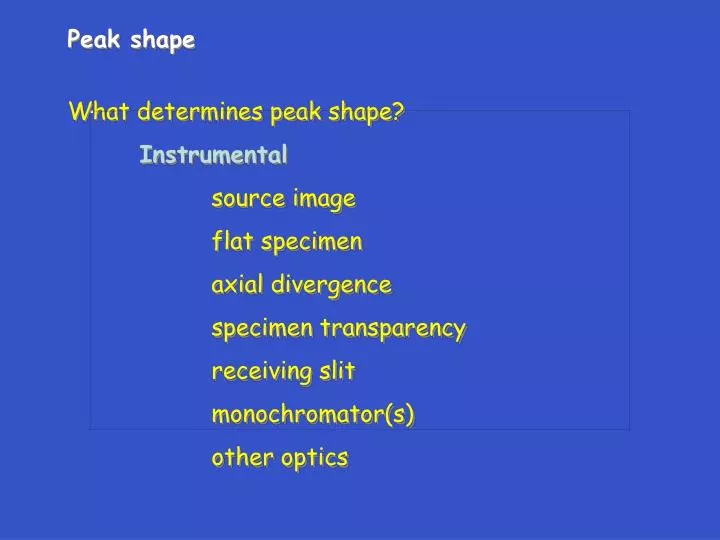
Peak shape What determines peak shape? Instrumental source image flat specimen axial divergence specimen transparency receiving slit monochromator(s) other optics
Peak shape What determines peak shape? Spectral inherent spectral width most prominent effect - Ka1 Ka2 Ka3 Ka4 overlap
Peak shape What determines peak shape? Specimen mosaicity crystallite size microstrain, macrostrain specimen transparency
Peak shape Basic peak parameter - FWHM Caglioti formula: H = (U tan2 + V tan + W)1/2 i.e., FWHM varies with , 2
Peak shape Basic peak parameter - FWHM Caglioti formula: H = (U tan2 + V tan + W)1/2 (not Lorentzian) i.e., FWHM varies with , 2
Peak shape 4 most common profile fitting fcns
(z) = ∫ tz-1 et dt 0 Peak shape 4 most common profile fitting fcns
Peak shape 4 most common profile fitting fcns
Peak shape X-ray peaks usually asymmetric - even after a2 stripping
Peak shape Crystallite size - simple method Scherrer eqn. Bsize = (180/π) (K/ L cos ) Btot = Binstr + Bsize 2 2 2
Peak shape Crystallite size - simple method Scherrer eqn. Bsize = (180/π) (K/ L cos ) 104Å Bsize = (180/π) (1.54/ 104 cos 45°) = 0.0125° 2 103Å Bsize = 0.125° 2 102Å Bsize = 1.25° 2 10Å Bsize = 12.5° 2
Peak shape Local strains also contribute to broadening
Peak shape Local strains also contribute to broadening Williamson & Hall method (1953) Stokes & Wilson (1944): strain broadening - Bstrain = <>(4 tan ) size broadening - Bsize = (K/ L cos )
2 2 2 2 Peak shape Local strains also contribute to broadening Williamson & Hall method (1953) Stokes & Wilson (1944): strain broadening - Bstrain = <>(4 tan ) size broadening - Bsize = (K/ L cos ) Lorentzian (Bobs − Binst) = Bsize + Bstrain Gaussian (Bobs − Binst) = Bsize + Bstrain
Peak shape strain broadening - Bstrain = <>(4 tan ) size broadening - Bsize = (K/ L cos ) Lorentzian (Bobs − Binst) = Bsize + Bstrain (Bobs − Binst) = (K / L cos ) + 4 <ε>(tan θ) (Bobs − Binst) cos = (K / L) + 4 <ε>(sin θ)
Peak shape (Bobs − Binst) cos = (K / L) + 4 <ε>(sin θ)
Peak shape (Bobs − Binst) cos = (K / L) + 4 <ε>(sin θ) For best results, use integral breadth for peak width (width of rectangle with same area and height as peak)
x y z y Peak shape Local strains also contribute to broadening The Warren-Averbach method (see Warren: X-ray Diffraction, Chap 13) Begins with Stokes deconvolution (removes instrumental broadening) • h(x) = (1/A) ∫ g(x) f(x-z) dz (y = x-z) h(x) g(z) f(y)
x y z y Peak shape Local strains also contribute to broadening The Warren-Averbach method h(x) & g(z) represented by Fourier series Then F(t) = H(t)/G(t) • h(x) = (1/A) ∫ g(x) f(x-z) dz (y = x-z) h(x) g(z) f(y)
Peak shape Local strains also contribute to broadening The Warren-Averbach method h(x) & g(z) represented by Fourier series Then F(t) = H(t)/G(t) F(t) is set of sine & cosine coefficients
Peak shape Local strains also contribute to broadening The Warren-Averbach method Warren found: Power in peak ~ ∑ {An cos 2πnh3 + Bn sin 2πnh3} An = Nn/N3 <cos 2πlZn> h3 = (2 a3 sin )/ n
Peak shape Local strains also contribute to broadening The Warren-Averbach method Warren found: Power in peak ~ ∑ {An cos 2πnh3 + Bn sin 2πnh3} An = Nn/N3 <cos 2πlZn> h3 = (2 a3 sin )/ sine terms small - neglect n
Peak shape Local strains also contribute to broadening The Warren-Averbach method Warren found: Power in peak ~ ∑ {An cos 2πnh3 + Bn sin 2πnh3} An = Nn/N3 <cos 2πlZn> h3 = (2 a3 sin )/ n = m'- m; Zn - distortion betwn m' and m cells Nn = no. n pairs/column of cells n
Peak shape • Local strains also contribute to broadening • The Warren-Averbach method • Warren found: • Power in peak ~ ∑ {An cos 2πnh3 + Bn sin 2πnh3} • An = Nn/N3 <cos 2πlZn> • W-A: • AL = ALS ALD (ALS indep of L; ALD dep on L) • L = na n
Peak shape • W-A showed • AL = ALS ALD (ALS indep of L; ALD dep on L) • ALD(h) = cos 2πL <L>h/a
Peak shape • W-A showed • AL = ALS ALD (ALS indep of L; ALD dep on L) • ALD(h) = cos 2πL <L>h/a • Procedure: • ln An(l) = ln ALS -2π2 l2<Zn2> n=0 n=1 n=2 ln An n=3 l2
Advantages vs. the Williamson-Hall Methodハ・Produces crystallite size distribution.・More accurately separates the instrumental and sample broadening effects.・Gives a length average size rather than a volume average size.Disadvantages vs. the Williamson-Hall Methodハ・More prone to error when peak overlap is significant (in other words it is much more difficult to determine the entire peak shape accurately, than it is to determine the integral breadth or FWHM).・Typically only a few peaks in the pattern are analyzed.