Download

1 / 21
230 likes | 412 Views
Path following control system for a tanker ship model. Lu’ cia Moreiraa, Thor I. Fossenb, C. Guedes Soaresa, 指導教授 : 曾慶耀 學生 : 曾彥翔 學號 10253081. Outline. 1.Introduction 2.Model 3.Controler. Introduction. The use of autonomous marine vehicles for differentapplications is growing

E N D
Path following control system for a tanker ship model Lu’ cia Moreiraa, Thor I. Fossenb, C. Guedes Soaresa, 指導教授:曾慶耀 學生:曾彥翔 學號10253081
Outline 1.Introduction 2.Model 3.Controler
Introduction • The use of autonomous marine vehicles for differentapplications is growing • Autonomous guidance and control technologies applied to marine vehicles are recognized as considerably important to the objective of achieving reliable and lowcost vessel • control systems must be able to navigate in multiple mission or test scenarios.
In this paper simulations are presented in order to demonstrate the performance of the guidance and control design for the model of the ‘‘Esso Osaka’’ tanker
Traditionally, trajectory tracking control systems for autonomous vehicles are functionally divided into three subsystems: guidance, navigation and control • The solution adopted here was to design a conventional autopilot controlling the heading ψ and a speed controller controlling the vehicle’s speed u in combination with a line of-sight (LOS) algorithm
Model (1).Coordinate frames • Themoving coordinate frames conveniently fixed tothe vehicle and is called the body-fixed reference framewith the center of gravity (CG)
η:denotes the position and orientation vector with coordinates in the earth-fixed frame, ν:denotes the linear and angular velocity vector with coordinates in the body fixed frame τ:is used to describe the forces and moments acting on the vehicle in the body-fixed frame.
The model was scaled 1:100from the real ‘‘Esso Osaka’’ ship.
the current’s magnitude the current’s spatial direction the ship’s heading angle the ship’s spatial forward component of velocity over the ground the ship’s spatial transversecomponent of velocity the forward component of relativevelocity the transverse component of relative velocity And civen by
The derivatives with respect to time of u and v are given by the following expressions with the derivatives with respect to time of , and given by
(2).Control plant model In order to design the steering autopilot becomes necessary to simplify the mathematical model described in the previous section in a 2 DOF (sway–yaw) linear maneuvering model A linear maneuvering model is based on the assumption that the cruise speed of the ship u is kept constant(u=constant) while v and r are assumed to be small. A 2 DOF nonlinear maneuvering model can be expressed by
is the system inertia matrix, is the Coriolis centripetal matrix, is the damping matrix The resulting model then becomes
Nomoto et al. (1957) proposed a linear model for the ship steering equations that is obtained by eliminating the sway velocity, that named Nomoto’s second order model by r and δ and by then Neglecting the roll and pitch modes
The values obtained for K and T of the first order Nomoto model, considering a speed u0 equal to 0.4 m/s, are:
Controller • PID heading controller Assuming that ψ is measured by using a compass, a PID controller is is the controller yaw moment, is the heading error, (<0) is the proportional gain constant, (<0) is the derivative time constant, (<0) is the integral time constant
A continuous-time representation of the controller is Where then
(2) Autopilot reference model An autopilot must have both course-keeping and turning capabilities. This can be obtained in one design by using a reference model to compute the desired states , , and needed for course-changing (turning) wile course-keeping, that is can be treated as a special case of turning. A simple third order filter for this purpose is where the reference is the operator input, In this case on = 0.45 rad/s and critical damping ξ =1 were considered
(3) Speed controller using state feedback linearization The basic idea with feedback linearization is to transform the nonlinear systems dynamics into a linear system Combining the model of the ship in surge is given by
The commanded acceleration can be calculated through the speed controller can be computed by