Download
1 / 39
390 likes | 513 Views
15. Firms, and monopoly. Varian, Chapters 23, 24, and 25. The firm. The goal of a firm is to maximize profits Taking as given Necessary inputs Costs of inputs Price they can charge for a given quantity We will ignore inputs for this course (Econ 102, or I/O will cover this).

E N D
15. Firms, and monopoly Varian, Chapters 23, 24, and 25
The firm • The goal of a firm is to maximize profits • Taking as given • Necessary inputs • Costs of inputs • Price they can charge for a given quantity • We will ignore inputs for this course (Econ 102, or I/O will cover this)
Standard theory • Intuition • Firm chooses a price, p, at which to sell, in order to maximize profits • Our approach today • The firm chooses a quantity, q, to sell • Inverse demand function is given p(q)
Firm decision in the short run Max p(q)q– c(q) • Differentiate wrtq and set equal to zero: MR = MC p(q) + qp’(q) = c’(q) Cost Revenue, R(q) = p(q)q Marginal cost Revenue from extra unit sold Revenue lost on all sales due to price fall
Perfect competition (many firms) Max p(q)q– c(q) • Perfect competition: p(q) = p p=MR = MC p+ 0 = c’(q) Cost Revenue, R(q) = p(q)q Marginal cost Revenue from extra unit sold Firm is too small to affect price
Pricing in the short run Perfect competition: • p = 20 • c(q) = 62.5+10q+0.1q2 • Find the firm’s profit-maximizing q Monopolist • p(q)= 50 - 0.1q • c(q) = 62.5+10q+0.1q2 • Find the firm’s profit-maximizing q
Cost function definitions c(q) = 62.5+10q+0.1q2 • Fixed cost: the part of the cost function that does not depend on q • Variable cost: the part of the cost function that does depend on q • Total cost: FC+VC • Average total cost: (FC+VC)/q=c(q)/q
How many firms will there be? p Perfect competition • In long run, competition forces profits to 0 • P = ATC(q) • P = MC(q) • C’(q) = C(q)/q • Solve for q ATC MC q
How many firms will there be? p Perfect competition • Knowing q • P = MC(q) • Q=D(P) • #firms = Q/q ATC MC D(p) q
The long run outcome Perfect competition: • D(P) = 600 - 20P • c(q) = 62.5+10q+0.1q2 • Find the long run q • Find the long run price, and # of firms Natural monopoly: • D(P) = 600 - 20P • c(q) = 640+10q+0.1q2 • What is q when MC=ATC? • How many firms will there be?
Natural monopoly p • D(p)<q at p where MC=ATC • Happens when fixed cost high relative to • marginal cost • inverse demand • Fixed cost can only be covered by p>MC ATC MC D(p) q
Monopolist • Natural monopolies • Electricity • Telephones • Software? • Monopoly can also be by government protection • Patented drugs • Imposed with violence • Snow-shovel contracts in Montreal
Monopolist • No competition • Monopolist free to choose price • MR(q) no longer constant p • Single price: set MR(q) = MC(q) • More elaborate pricing schemes to follow • Price discrimination
Monopoly pricing (no price discrimination) • Note: When demand is linear, so is marginal revenue • P = A – Bq • MR = A – 2Bq pm Profit MC Demand MR qm Optimal quantity set by monopolist
Inefficiency of monopoly Dead weight loss pm Mark-up over Marginal cost MC Demand MR qm q*
(Price) elasticity of demand • The elasticity of demand measures the percent change in demand per percent change in price: e = -(dq/q) / (dp/p) = -(p/q)*(dq/dp) < 0
Optimal mark-up formula p(q) + qp’(q) = c’(q) can be rearranged to make: p = MC / (1 – 1/|e|) This can be rearranged to yield: (p – MC)/MC = 1 / (|e| - 1) > 0
Demand elasticity p p Elasticity > 1 Elasticity = 1 Constant elasticity of demand Elasticity < 1 q q p = q -e p = a - bq
Monopolist’s decision Natural monopoly: • D(P) = 600 - 20P • c(q) = 640+10q+0.1q2 • What q will monopolist choose? • What is their profit? • What is elasticity of demand at this price/quantity?
Price discrimination • Idea is to charge a different price for different units of the good sold • What does “different units” mean • Purchased by different people • E.g., children, students, pensioners, military • Different amounts purchased by a given person • E.g., quantity discounts, entrance fees, etc.
Three degrees of discrimination • First degree PD • Each consumer can be charged a different price for each unit she buys • Second degree PD • Prices can change with quantity purchased, but all consumers face the same schedule • Third degree PD • Prices can’t vary with quantity, but can differ across consumers
First degree PD • Outcome is • Pareto efficient • Consumer earns • no consumer • surplus Profit of fully discriminating monopolist MC = c • Alternative pricing mechanism: If you buy x units, you pay a total of T + cx Profit of non- discriminating monopolist Demand x* xm Entry fee
With more than one consumer... ….charge a different entry fee to each ….but the same marginal price Profit from consumer A Profit from consumer B MC = c MC = c Demand Demand x*A x*B Consumer B Consumer A
Entry fees as “two-part-tariffs” • Let A’s consumer surplus be TA and let B’s be TB . • Monopolist sets a pair of price schedules: Consumer B RB = TB + cx Consumer A RA = TA + cx Entry fees Price per unit = c
Second degree PD • Suppose again there are two types of people – A-types and B-types • Half is A-type, half B-type • …but now we cannot tell who is who • Can the monopolist still capture some of the consumer surplus? Yes - airlines • All of it? No
A problem of information…. TA A’s demand • Best pricing policy: Offer two options: Option A: x*Afor $(U+V+W)+cx*A Option B:x*Bfor $U+cx*B • But then A would choose option B • She gets surplus V from option B, and 0 from option A • Monopolist gets profit U B’s demand TB V W U MC x*A x*B x
R Option A Option B is better than option A for person A RA RB Option B x x*B x*A
The monopolist can do a little better…. A’s demand • Option A’: x*Afor $(U+W)+cx*A • A will be happy to take this offer • She gets a surplus of V • Monopolist gets profit U+W B’s demand V W U MC x*A x*B x
…but it can do even better A’s demand • Option A’’: x*Afor $(U+W+DW)+cx*A • Option B’’ x’’Bfor $(U-DU)+cx’’B • A still willing to take option A’’ over option B’’ • Profit up by DW-DU DW B’s demand V W U MC DU x*A x*B x x’’B
…and the best it can do is? Gain from higher fees paid by A-types from further decreasing x+B A’s demand • Stop when = B’s demand Loss from lost sales to B-types from further decreasing x+B V W U MC x*A x*B x x+B
Should the monopolist bother selling to low-demand consumers? Going further, you lose more on the B-types than you gain on the A-types Going all the way to zero, you lose less on the B-types than you gain on the A-types YES: Sell to B-types NO: Sell only to A-types MC MC A A B B x+B x+B=0 x*A x x*A x
2nd degree price discrimination High type: • DH(P) = 100 - P Low type: • DH(P) = 70 – P • MC=10 • What bundles should the monopolist offer? • At what prices?
2nd degree price discrimination High type: • DH(P) = 100 - P Low type: • DH(P) = X – P • MC=10 • For what value of X will the monopolist not sell to low types?
Outcome B-types • They buy less than the Pareto efficient quantity: x+B < x*B • They earn zero consumer surplus A-types • They buy the Pareto optimal amount, x*A • They earn positive consumer surplusFN • this is always what they could earn if they pretended to be B-types FN: Whenever x+B >0
Third degree price discrimination • Monopolist faces demand in two markets, A and B • Suppose marginal cost is constant, c • Then the monopolist just sets prices so that pA = c / (1 – 1/|eA|) pB = c / (1 – 1/|eB|)
Some problems • Non-constant marginal cost? • Replace c above with c’(xA+xB) • What if demands are inter-dependent? • E.g., xA(pA,pB) and xB(pB,pA) • Applications • Peak-load pricing • A:Riding the metro in rush-hour • B: Riding off-peak • Children’s and adults’ ticket prices
Bundling • Suppose a monopolist sells two (or more) goods • It might want to sell them together – that is, in a “bundle” • E.g.s • Software – Word, PowerPoint, Excel • Magazine subscriptions
Software example Two types of consumer who have different valuations over two goods Assume marginal cost of production is zero
Sell separately Highest price to sell 2 word processors is 100 Highest for spreadsheet is 100 Sell two of each, for profit of 400 Bundle Can sell a bundle to each consumer for 220 Total profit is 440 Dispersion of prices falls with bundling Selling strategies