Download
1 / 33
330 likes | 406 Views
Topic 13. Lecture 19. Mode of Reproduction, Population structure, Drift Factors of Microevolution: 1) Mutation 2) Selection 3) Mode of reproduction 4) Population structure 5) Random drift

E N D
Topic 13. Lecture 19. Mode of Reproduction, Population structure, Drift Factors of Microevolution: 1) Mutation 2) Selection 3) Mode of reproduction 4) Population structure 5) Random drift Mutation and selection are the two most important factors of Microevolution - even theoretically, Darwinian evolution cannot occur without either of them. However, the other 3 factors also cannot be ignored, because they strongly affect how evolution occurs in nature.
3) Mode of Reproduction Reproduction is characterized by two things: 1) how many cells initiate an offspring and 2) what kinds of cellular processes initiate an offspring. Unicellular channels Vegetative reproduction by many cells is common, but almost never occurs without single-cell reproduction.
Sex Asexual reproduction, or apomixis, origination of an offspring from a single mitotically produced cell, only rarely represents the only mode of reproduction in eukaryotes. Bdelloid rotifers are apparently 100% apomictic. Amphimictic life cycle is universal, because n and 2n phases always alternate strictly - there are no (?) cases of n>2n>4n>2n>n (S>S>M>M) cycles. Still, a lot of variation is known within this framework. This variation is concerned with what happened in each phase (reduced-unreduced), whether there are physical connections between organisms representing different phases, and how asexual reproduction is incorporated.
In red algae, there is a regular succession of two different individuals, carsporophyte and tetrasporophyte, within the 2n-phase. In Polysiphonia, carposporophyte lives on gametophyte (as in mosses). Different sandwich organisms are known in other red algae.
The most profound reduction of the n-phase occurs in ciliates, where this phase is reduced below the cell level, to a "naked" nucleus. In animals n-phase of always reduced, except 7 groups with haploid males (Hymenoptera, stick insects, 3 clades of mites, 2 clades of beetles). In contrast, in green plants n-phases is never reduced to the level of individual cells. Crossing-over can be absent in one sex (heterogametic), but never, as far as we know, in both sexes.
The impact of sex on the population is due to three "subfactors": a) Mendelian segregation Randomization of the 2n-phase - Hardy-Weinberg law b) recombination (due to two mechanisms) Randomization of joint distributions of alleles at different loci c) system of mating Possible deviations from Hardy-Weinberg law Let us consider them separately.
3a) Mendelian segregation Mendelian segregation affects only the diploid phase. Mendelian segregation in spermatogenesis and oogenesis. Let us assume that gametes unite randomly. Then, the frequencies of diploid genotypes in the next generation are connected to the frequencies in the current generation as follows: 1) allele frequencies remain the same and 2) alleles become independently distributed among the genotypes. This fact is called Hardy-Weinberg law.
In the simplest case of just two alleles, A and a, Hardy-Weinberg frequencies of the three diploid genotypes AA, Aa, and aa, are related to the allele frequencies [A] and [a] in the following way: [AA] = [A]2, [Aa] = 2[A][a], [aa] = [a]2 Because [A] + [a] = 1, this implies that [AA] +[Aa] + [aa] = 1, as expected. Of course, this is just another way of saying that [A] and [a] are distributed independently among the diploid genotypes. Independent distribution of alleles in the diplophase is established instantly, after just one generation. We can start from a completely homozygous population ([AA] = [aa] = 0.5) or from a completely heterozygous population ([Aa] = 1), and in both cases the next diplophase will conform to Hardy-Weinberg genotype frequencies for [A] = 0.5, and will have 25% of individuals with genotypes AA and aa each, and 50% of individuals with genotype Aa. Two mechanisms can lead to random union of gametes: 1) all the gametes form one pool and then unite randomly or 2) diploid individuals mate randomly and then gametes unite randomly within each pair. Mechanism 1) must leads to Hardy-Weinberg frequencies of diploid genotypes by definition. Let us see how mechanism 2) ("2-step randomness") leads to the same result.
Consider an arbitrary set of genotype frequencies [AA], [Aa], and [aa] in the current diploid phase, with the current allele frequencies [A] = [AA] + 0.5[Aa] and [a] = [aa] + 0.5[Aa]. The Table lists the 6 possible matings between diploids (there is no need to distinguish reciprocal matings, such as AA x aa and aa x AA), together with their probabilities, when mating is random, and fractions of offspring of the 3 possible genotypes after each mating. Mendelian segregation in matings of diploids Mating Frequency Frequencies of offspring within a mating AA Aa aa AA x AA [AA]2 1 0 0 AA x Aa 2[AA][Aa] 1/2 1/2 0 AA x aa 2[AA][aa] 0 1 0 Aa x Aa [Aa]2 1/4 1/2 1/4 Aa x aa 2[Aa][aa] 0 1/2 1/2 aa x aa [aa]2 0 0 1 Now we can calculate frequencies of diploid genotypes in the next generation, as the following sums: [probability of a mating] x [probability of this mating producing an offspring with a particular genotype]. For example, [AA]t+1 = 1[AA]2+0.5(2[AA][Aa])+0(2[AA][aa])+0.25[Aa]2+0(2[Aa][aa])+0[aa]2 We can see that [AA]t+1 can be also expressed as ([AA] + 0.5[Aa])2, i. e. that [AA]t+1 = [A]2. Analogous calculations can be performed for the other two genotypes. Of course, [A]t+1 = [A], since segregation is Mendelian and there is no selection, all frequencies cannot change (check this). Hardy-Weinberg law works for any number of alleles. After Mendelian segregation and random gamete assortment, frequency of zygotes AiAj is 2[Ai][Aj] if i ≠ j and [Ai]2 if i = j.
3b) Recombination The coefficient of recombination between two loci, r, is the probability that alleles at these loci will be transmitted by a diploid organism in combinations different from how they were obtained from the parents. Frequencies of meiospores produced by a diploid that originated from gametes AB and ab. rAB = 0.5 if A and B are located on different chromosomes. The coefficient of recombination between a pair of loci located on the same chromosome is always below 0.5, and equals to the probability of the odd number of chiasmata between the loci. If loci A, B, and C are located, in this order, on the same chromosome close to each other, approximately rAC = rAB + rBC.
A Jack Jumper ant (Myrmecia pilosula). Its genome (haploid) consists of just 1 chromosome! Females are diploid, and males are haploid. Crossing-over depends on a very complicated molecular mechanism, comparable to DNA replication and repair, which operates before meiosis and in its early stages. Usually there are slightly more than 1 cross-overs per chromosome. Crossing-over is not required for cell functioning. Indeed, in many organisms, such as D. melanogaster male, crossing-over is absent, but meiosis is normal.
Let us find out how recombination affects genotype frequencies in haploids. Consider the simplest case of two loci with two alleles each, with an arbitrary set of haploid genotype frequencies [AB], [Ab], [aB], and [ab]. Recombination will reshuffle genotypes in meioses which will follow syngamies of only two types, since reshuffling requires both loci to be heterozygous. Syngamy Frequency Frequencies of meiospores after a syngamy AB Ab aB ab AB x ab 2[AB]x[ab] (1-rAB)/2 rAB/2 rAB/2 (1-rAB)/2 Ab x aB 2[Ab]x[aB] rAB/2 (1-rAB)/2 (1-rAB)/2 rAB/2 Taking into account effects of these two syngamies, we can calculate the 4 genotype frequencies in the next haploid phase: [AB]t+1 = [AB] + 2[AB]x[ab]{(1-rAB)/2-1/2} + 2[Ab]x[aB]{(rAB/2} = [AB] - [AB][ab]rAB + [Ab][aB]rAB = [AB] - DxrAB [Ab]t+1 = [Ab] + DxrAB [aB]t+1 = [aB] + DxrAB [ab]t+1 = [ab] - DxrAB And coefficients of association in the successive generations are connected by: Dt+1 = [AB]t+1[ab]t+1 - [Ab]t+1[aB]t+1 = = [AB][ab]-DrAB{[AB]+[ab]}+{DrAB}2-[Ab][aB]-DrAB{[Ab]+[aB]}-{DrAB}2 = D(1-rAB)
Thus, even free recombination (rAB = 0.5), together with random assortment of gametes, does not immediately lead to independent distribution of alleles at different loci. Instead, the coefficient of association declines only asymptotically, by 50% each generation.
3c) Non-random union of gametes Non-random union of gametes can be of the following types: i) Assortative mating - union based on similarity. Can cause excess (positive assortative mating) or deficit (negative a. m.) of homozygotes. ii) Inbreeding - union based on relatedness. Causes excess of homozygotes. iii) Anisogamy - union based on gametes size. Does not affect the population, as long as genotype frequencies are the same within both sexes. iv) Self-incompatibility - union based prohibition of syngamy for some genotypes. Apparently, its main impact is to prevent inbreeding. Sex (amphimixis) also can exist without any sexes, if every two gametes can form a zygote (for example, in some fungi).
Sex of the gamete can be determined by either the n-phase or the 2n-phase.
Self-incompatibility can coexist with anisogamy (angiosperms), or can exist separately (basidiomycetes, ciliates). In the most common system of angiosperm self-incompatibility, a pollen grain must not carry either of the two alleles of self-incompatibility locus S that are present in pistil (n-2n incompatibility).
4) Population structure 4a) Age structure Age structures vary from absent, when generations are discrete and nonoverlapping, to extremely complex, when a male can breed with his great-great-great-...-grandmother. Arabidopsis thaliana. Annual, seeds do not last long. Perch Perca fluviatilis. Reaches maturity at 2-3 years, can live and reproduce for over 20 years. Fresh-water copepod Eudiaptomus graciloides. Its eggs can remain in the state of diapause for decades. However, age structure of a population usually affects its Microevolution only marginally. Instead of specifying functions l(y), the probability of reaching an age y and m(y), fecundity at age y fitness still can be approximated by one number even when there is an age structure.
This one-number representation of fitness can be done in two ways: Life-time reproductive success: Malthusian parameter, the only root of Euler's equation: Malthusian parameter describes changes of the number of individuals in a population where everyone is characterized by the same l(y) and m(y). We can calculate R or, preferably, l, for each genotype, and use it as its fitness. Unless selection is very strong and fluctuates in time widely, individuals of different ages are characterized by approximately the same genotype frequencies. Thus, approximate description of an age-structured population which ignores this structure usually works.
4b) Spatial structure Spatial structure of a population often cannot be ignored - because movements in space may be restricted, in contrast to movements in time, and genotype frequencies in different parts of the range of the population can be very different. In the extreme case when individuals in different areas evolve independently, due to lack of dispersal, each area is treated as a separate population. However, there are many intermediate situations, when dispersal is restricted but not absent, and we need to consider spatial structure explicitly. Distribution of the B type blood allele in native populations of the world
This can be important in two cases. First, environmental conditions, and directions of selection can be different in different locations, connected by limited dispersal. A famous example is the presence of S hemoglobin alleles in human populations that live in areas where malaria is very common. This allele is selected against in areas where malaria is rare or absent.
Second, limited dispersal can slow down the expansion of a beneficial mutation, which needs time to take over the whole range, starting from the place of its origin. Global Spread of Chloroquine-Resistant Strains of Plasmodium falciparum. Still, on long time intervals, spatial structure is not crucially important for Microevolution, because eventually a substantially advantageous mutation will take over the whole population.
5) Genetic drift We cannot postpone dealing with this factor of Microevolution any longer. Finally, we need to face the reality: changes of a population are not deterministic but stochastic (unpredictable and irreproducible). Sometimes the inherent stochasticity of nature can be ignored, but often this is impossible. Genetic drift (or random genetic drift) is not the only reason for stochasticity of Microevolution. There are at least two other reasons: 1) stochasticity of mutation. A particular mutation may occur only once in may generations in the population, at unpredictable moments. 2) unpredictable changes of fitness, due to changes of the external conditions. Still, genetic drift operates in every population and strongly affects evolution at loci where selection is weak or absent.
What is genetic drift? It is a process of stochastic changes of genotype frequencies, due to unpredictability of reproduction at the level of individuals. Can we imagine a population without genetic drift? Yes, if every asexual individual leaves exactly one offspring, there would be no drift. However, this is impossible. Even if there are no systematic differences between fitnesses of genotypes, so that the expected number of offspring of each individual is the same, the actual numbers of offspring of different individuals will be different.
In sexual populations, genetic drift also occurs due to stochasticity of Mendelian segregation in heterozygous individuals. Even if every mating produces exactly two offspring, genotype frequencies would change in a sexual population. We can think of the gene pool of the next generation as a SAMPLE from the current gene pool.
Genetic drift leads to random changes of allele frequencies within a population. These changes occur faster in small populations. Let us consider the simplest case of two alleles, A and a. Allele frequencies of an infinitely large asexual populations would not be affected by genetic drift and, thus, would remain constant.
If genetic drift acts alone for a long period of time, it keeps increasing the variance of the distribution of allele frequencies within the population. However, in contrast to selection, genetic drift does not affect the expected (mean) allele frequencies.
After a long enough time, there is a large probability that one of the alleles already became fixed. If this did not yet happened, surprisingly, the probability of all other (different from 0 and 1) allele frequencies is the same at every moment (flat distribution). Eventually, variation will be lost, and allele A will reach fixation with probability f (and allele a will reach fixation with probability 1-f), where f is the initial frequency of allele A.
One can say that, without mutation, 0 and 1 are absorbing states, in random drift of an allele frequency.
Effective population size Can we characterized the intensity of random drift within a population by one number? Yes, this is often possible, and this number is called effective population size, Ne. Effective size of a real population is the size of idealized Wright-Fisher population in which random drift proceeds at the same rate as it does in our real population. What is the "rate" of genetic drift? We will consider the variance effective size, so that the rate will be the variance of genotype frequency introduced by genetic drift. What is Wright-Fisher population? Assume that there are N (haploid) individuals. Each of them produces very many "provisional offspring", and N actual offspring are recruited randomly from them.
In such a population, the probability q of an individual having k offspring has Poisson distribution with the parameter (both mean and variance) 1: q(k) = e-11k/k! If the number of individuals of some genotype A among parents is K, the number of such individuals among offspring, O, has binomial distribution (we need to consider the whole distribution because the process is stochastic): The variance of the distribution of [A]t+1, frequency of A among the offspring is [A](1-[A])/N, where [A] = K/N is the frequency of A among parents, as well as the expected frequency of A among offspring. Drift is a fair process! Thus, Ne = [A](1-[A])/{variance of the distribution of D[A]} where D[A] = [A]t+1-[A] is a change of genotype frequency in one generation.
Usually, effective size of a natural population is much smaller than the actual size (head count). This is what is always observed in nature, due to population bottlenecks (episodes of low population size) and wide variation in the number of offspring between individuals. Poisson distribution of this number, a property of Wright-Fisher model, has a much smaller variance than the corresponding distributions in nature. However, theoretically, Ne > N is also possible. Ne = infinity Ne = 2N
Quiz Study experimentally genetic drift that is caused by Mendelian segregation only. Consider a population of diploids, with a constant size N = 4. Individuals are hermaphrodite, monogamous outcrossers, mate randomly, and each pair produces 2 offspring. Generations are discrete. Initially, all the four individuals are heterozygous, with alleles A and a (only 1 locus is considered). Do the following: 1) Decide who mates who. It is enough to find a partner for individual number 1. For this purpose, roll two coins, and use binary representation of numbers 1, 2, 3, and 4 (heads of both coins mean 1, head of coin 1 and tail of coin 2 means 2, tail of coin 1 and head of coin 2 means 3, and tails of both coins means 4). If you get heads of both coins, roll them again. After you determine the partner for individual 1, the remaining two have to mate each other. 2) Determine genotypes of offspring one-by-one. Offspring 1 is the 1st offspring from the 1st pair. If a parent is homozygous, it will transmit its only allele. If a parent is heterozygous, it will transmit either A or a with probability 0.5 - roll a coin to determine which one is transmitted. This way, create genotypes of all the 4 offspring, and start the next generation. 3) Put all the data in a table. Run this experiment at least 3 times, each time until either allele is fixed. Plot the trajectories of allele frequencies. Calculate the average number of generations until fixation.