Download
1 / 17
170 likes | 323 Views
A physical basis of GOES SST retrieval. Prabhat Koner Andy Harris Jon Mittaz Eileen Maturi. Summary. One year match up database ( Buoy & Satellite) has been analyzed to understand the retrieval problem of satellite measurement.

E N D
A physical basis of GOES SST retrieval PrabhatKoner Andy Harris Jon Mittaz Eileen Maturi
Summary • One year match up database ( Buoy & Satellite) has been analyzed to understand the retrieval problem of satellite measurement. • Various forms of errors and ambiguities for SST retrieval will be discuused. • 110,000 night only data (GOES12 & Buoy) has been considered from this database to compare results with different choices of solution processes: • RGR -> Regression • OEM -> (KTSe-1K+Sa-1)-1KTSe-1ΔY • ML -> (KTSe-1K)-1KTSe-1ΔY • RTLS -> (KTK+λR)KTΔY (Regularized Total Least square) • 3.9 & 10.7 μm -> 2 channel • 3.9, 10.7 & 13.3 μm -> 3 channel • Two variables of SST & TCWV
Nomenclature X -> state space parameters Y -> Measurements ΔY -> Residual (Measurements – forward model output) ΔX -> Update of state space variables δY -> Measurement noise δX -> Retrieval error Sa -> a priori/ background covariance Se -> measurement error covariance K -> Jacobian (derivative of forward model) κ(K) -> condition number of Jacobian (highest singular value/lowest singular value) T -> Brightness temperature in satellite output BT -> Calculated Brightness temperature SSTg-> Sea Surface Temperature First Guess SSTb -> Sea Surface Temperature from Buoy measurement SSTrgr -> Sea Surface Temperature retrieval using regression SD -> Standard Deviation RMSE -> Root Mean Square Error.
Historical Regressed based SST retrieval SSTrgr=C0+∑Ci Ti ; C=a+b{sec(θ)-1}+… Alternately we can use radiative transfer physics inverse model Coefficients are derived from in situ buoy data or L4 bulk SST. Validate with Buoy data Bulk SST from Satellite measurement?
Physical Retrieval Statistical (OEM) Deterministic (TLS) A posteriori observation A priori First we will see Pros-con of OEM Data & Measurement both uncertain It can only estimate a posteriori probability density (parameters x’: “Best Guess”) by calculating Maximum likelihood P(x|y). Measurement only uncertain Jacobian error is condidered in cost funtion minimization. Retrieval in pixel level
Shortcomings of OEM Global SST distributions match quite well, but… …large differences between 1st guess and buoy SST are real A-priori based cloud screening algorithm (CSA) in place to constrain in image data
Paradox of OEM output To further investigate this issue, we calculate information content • OEM=(KTSe-1K+Sa-1)-1KTSe-1ΔY • Information comes from measurement and a priori covariance. • COV= (√Sa-1)-1ΔY • Sa= • By accident the choice Sa, COV retrieval is just adding residual of 3.9 μm channel with FG. • Covariance has no physical meaning • Add measurement increase noise into retrievals
Big Question? H=-0.5 ln(I-AVK) Two measurement cannot produce more than 2 pieces of information. OEM may be valid for linear problem, not applicable for inherently nonlinear RTE.
Condition number of Jacobian Difficulty solve using satellite data, drive to further investigation • The condition number of jacobian of most real life problem is high. Yields • δx <= κ (K) δy • K=randn(2); (κ(K) = 118) • x=randn(2,1); [-1.35 0.97] • y=K*x • For ii=1:100 • error(:,ii)=0.01*randn(2,1); • xrtv(:,ii)=K-1(y+error(:,ii)); • End Apart from model physics and measurement errors, the error due to κ(K) plays a role. (KTSe-1K+Sa-1)-1KTSe-1ΔY Remedies: Reducing the condition number of inverted matrix Regularization, constraints, scaling, weighting etc. We use RTLS method. Uniquely solved in simulation study.
Fast Forward Model Error Online monitor ECMWF It is not an instrument calibration problem or bias Need improvement of fast forward model.
Simulated Retrieval δx<= κ (K) δy
Quality Flagging Algorithm K=U∑VT -> Singular vector decomposition VT ∑1-1U ΔY ->Principle Component solution VT ∑n-1U ΔY ->Lowest singular value solution Lowest singular value solution increases error in retrieval where measurement noise is high. Difference of two solutions is able identified bad retrieval.
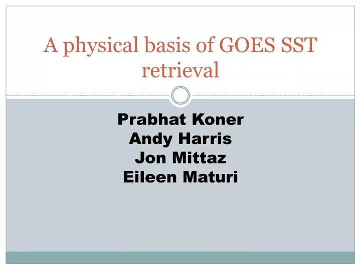
Comparative results Results are based on single iteration. Second iteration may further improve the results for physical retrieval. Same data and model, results are different due to choice of solution methods
Conclusions Radiativetransfer can be successful used in retrieval of SST from satellite data if we pursue rigorous physics (accurate RTM) and mathematics There is an ambiguity in the cost function minimization for nonlinear problems, i.e. (Yδ-KX)TSe-1(Yδ-KX) + (X-Xa)TSa-1(X-Xa) does not apply if Y ≠ KX
Few Definitions • Model: a simplified description of how the ‘real world’ process behaves • Forward Model : the set of rules (mathematical functions) that define the behaviour of the process (e.g. a set equation) Forward model of remote sensing • Well understood but mathematically complex function • Analytical derivative is almost impossible. • Stable: On some appropriate scale a small change in the input produces a small change in the output • Inverse Model: quantities within the model structure that need to be quantified from observation data Inverse model of remote sensing is ill-posed • Is the solution we find unique? • Observational, numerical and model errors often cause the inverse problem to be unstable: a small change in the input produces a large change in the output
Forward Model Intensity of the background source “Transmittance” between 0 and L “Transmittance” between l and L Emission term Absorption term Spectral intensity observed at L “Optical depth” “Absorption coefficient”
Forward Model “Line strength” “Line shape” “Cross section” “number density” “Volume Mixing Ratio” “Absorption coefficient” Spectral intensity observed at L GENSPEC: line shape: Voigt: line Strength: HITRAN 2004