Download

1 / 20
200 likes | 320 Views
Adaptive resolution of 1D mechanical B-spline. Julien Lenoir , Laurent Grisoni, Philippe Meseure, Christophe Chaillou. Problem. Real-time physical simulation of a knot. Fixed resolution simulation. Goal: adaptive resolution simulation. Related work. 1D model and knot tying

E N D
Adaptive resolution of 1D mechanical B-spline Julien Lenoir, Laurent Grisoni, Philippe Meseure, Christophe Chaillou
Problem Real-time physical simulation of a knot Fixed resolution simulation Goal: adaptive resolution simulation
Related work • 1D model and knot tying • [Wang et al 05] Mass-spring model, not adaptive • [Brown et al 04] Non physics based model, ‘follow the leader’ rules, not adaptive • Generality on multiresolution physical model • Discrete model: [Luciana et al 95, Hutchinson et al 96, Ganovelli et al 99] • Continuous model: [Wu et al 04, Debunne et al 01, Grinspun et al 02,Capell et al 02]
Outline • Physical simulation of 1D B-spline • Geometric subdivision of a B-spline • Mechanical multiresolution • Results • Side effect • Conclusion
Physical simulation of 1D B-spline • Geometric model: B-spline qk=(qkx,qky,qkz)position of the kth control points bkare the spline base functions tis the time, s the parametric abscissa • Physical model: Lagrange formalism Variational formulation + Mechanical system defined via DOF = Energy minimization relatively to DOFs
Physical simulation of 1D B-spline • Physical Model: • Definition of the DOFs:
Kinetic energy Energies not derived from a potential(Collisions, Frictions…) Potential energies (Deformations, Gravity…) Physical simulation of 1D B-spline • Physical Model: • Definition of the DOFs: • Lagrange equations applied to B-spline:
Physical simulation of 1D B-spline • Physical Model: • Definition of the DOFs: • Lagrange equations applied to B-spline: Generalized mass matrix: Gather the and terms
Physical simulation of 1D B-spline • Continuous deformation energies • Stretching [Nocent01]: • Green-Lagrange tensor allows large deformations • Piola-Kirchhoff elasticity constitutive law • Bending: in progress… • Twisting: not treated (need to extend the model to a 4D model)
Physical simulation of 1D B-spline • Constraints by Lagrange multipliers (λi): • Direct integration into the mechanical system:
Physical simulation of 1D B-spline • Constraints by Lagrange multipliers (λi): • Direct integration into the mechanical system: • λi links a scalar constraint g(s,t) to the DOFs
Time step Physical simulation of 1D B-spline • Constraints by Lagrange multipliers (λi): • Direct integration into the mechanical system: • λi links a scalar constraint g(s,t) to the DOFs • L and E are determined via the Baumgarte scheme: => Possible violation but no drift
Geometric problem Physical simulation of 1D B-spline Resulting physical simulation: - 6 constraint equations - 33 DOF Lack of DOF in some area
insertion Geometric subdivision of a B-spline • Exact insertion in NUB-spline (Oslo algorithm): NUBS of degree d Knot vectors: • The simplification of BSplines is often an approximation
Mechanical multiresolution • Insertion and suppression: • Reallocate the data structure: pre-allocation • Shift the pre-computed data and re-compute the missing part (example: , ) • Continuous stretching deformation energies: • Pre-computed terms: • 4D array • Sparse • Symmetric Avoid multiple computationStorage in an 1D array
Mechanical multiresolution • Criteria for insertion: • Geometric problem => geometric criteria • Problem appears in high curvature area • Fast curvature evaluation based on control points • Criteria for suppression: • Segment rectilinear
Results Low resolution Adaptive resolution High resolution
Side effect • Geometric property: • Multiple insertion at the same location decrease locally the continuity • => ‘Degree’ insertions= C-1 local continuity = Cutting • Mechanical property: • Dynamic cuttingwithout anythingspecial to handle
Side effect • Example of multiple cutting:
Conclusion • Real-time adaptive 1D mechanical model • Continuous model (in time and space)=> Stable over time=> Can handle sliding constraint [Lenoir04] • Dynamic cutting appears as a side effect • Future works: • Enhance the deformation energies: Better bending + Twisting (4D model, cosserat [Pai02]) • Handle length constraint