Download
1 / 28
280 likes | 285 Views
Developers: John Walker, Chris Jewett, John Mecikalski, Lori Schultz. Convective Initiation (CI) GOES-R Proxy Algorithm. University of Alabama in Huntsville (UAHuntsville). Satellite Detection. Radar Detection. Height (km). Time. Forecast without satellite.

E N D
Developers:John Walker, Chris Jewett, John Mecikalski, Lori Schultz Convective Initiation (CI) GOES-R Proxy Algorithm University of Alabama in Huntsville (UAHuntsville)
Satellite Detection Radar Detection Height (km) Time Forecast without satellite Forecast with satellite Motivation • Mecikalski & Bedka (2006) as initial methodology • Mecikalski et al. (2008, 2010a,b) • MacKenzie (2008) • Siewert (2008); Harris et al. (2010) • Siewert et al. (2010); Walker et al. (2011) (Longer lead time) 12 9 6 3
Purpose of Satellite-based CI Algorithm Satellites “see” cumulus before they become thunderstorms! t= –30 min t= –15 min t= Present By monitoring signals of cloud growth from satellite, CI can be forecast up to ~1.5 hours in the future. CI Time: First ≥35 dBZ echo on radar (at -100C)
Download latest GOES imagery Make Cloud Mask Produce AMVs Brief Algorithm Summary Track “Cloud Objects” from ‘T1’ to ‘T2’ Determine CI forecast for each tracked Cloud Object using 6 spectral/temporal differencing tests (aka: “Interest Fields”) Output CI forecast for each Cloud Object
The UAH CI algorithm currently employs a “Day-time” and a “Night-time” version. The main difference between them is the type of Cloud Maskused. Day-time: Advanced “Convective Cloud Type” algorithm used to define several types of clouds (Berendes et al, 2008), such as cumulus, towering cumulus, cumulonimbus, cirrus, stratus, etc. The input requires all available GOES channels (including “Visible”). Night-time: Regular “Cloud Mask” (no cloud types) generated from multi-day composites of GOES Infrared channels (Jedlovec and Haines, 2008). Brief Algorithm Summary
Day-time CCMask Classifications Used: -Cumulus -Tower Cumulus -Warm Water Cloud -Cold Water Cloud Object Omitted From Processing Mature Cloud Object Pre-CI/Immature Cloud Objects Object Tracking Methodology Night-time CMask Portions Used : -Any part of cloud mask > -20 C T1 Time 1= “T1” Time 2= “T2”
Assign unique Integer IDs to each object at T1. 1 Apply AMVs to objects at “T1” Object Tracking Methodology 2 3 T1
Advect T1 objects to projected locations at T2 1 1 Object Tracking Methodology 2 3 2 3
T1 Advected T2 Actual Object Tracking Methodology T2 T2
Look for overlap between Actual T2 objects and those projected from T1 Overlap Object Tracking Methodology Overlap Overlap
Where there is object overlap, have the “actual” T2 objects inherit the same, unique Integer ID number as at T1. 1 Object Tracking Methodology 2 3 The objects are now tracked! T2
Time 1 (T1) Object Tracking Methodology
Time 2 (T2) Object Tracking Methodology
A series of six* different “interest field” tests are performed for each tracked object, utilizing various available GOES channels: *13 tests will be used for the GOES-R algorithm 1 2 CI Interest Fields 3 4 5 6 Table from Mecikalski and Bedka 2006
Cloud-top Glaciation 1 Cloud-top growth 2 Cloud height, relative to mid-troposphere (Ackerman, 1996; Schmetz et al, 1997) CI Interest Fields 3 4 Cloud height (Inoue, 1997; Prata, 1989; Ellrod, 2004) 5 6 Cloud-top height changes Table from Mecikalski and Bedka 2006
-100 C 00 C Decreasing Temperature CI Interest Fields: EXAMPLES 10.7um Cooling Rate T1 T2 Increasing Time
CI Interest Fields: EXAMPLES 6.5-10.7um (WV – IR) Channel Difference Pressure (mb) Pressure (mb) Decreasing Temperature GOES 6.5um (WV) Weighting Function* GOES 10.7um (IR) Weighting Function* *Adapted from UW/CIMSS site
Example: WV – IR = -300C Channel differences <0 indicate cloud top height is less than the mid-troposphere height. The magnitude of this value indicates just how high the cloud top is, relative to the mid-troposphere. -250 C Pressure (mb) CI Interest Fields: EXAMPLES 6.5-10.7um (WV – IR) Channel Difference Decreasing Temperature 50 C
Example: WVT1 – IRT1 = -300C WVT2 – IRT2 = -200C T2 – T1= 10 Temporal differences >0 indicate cloud top is growing upward, toward the mid-troposphere. The magnitude of this value indicates just how fast the cloud top is growing. T1 T2 -250 C -250 C Pressure (mb) CI Interest Fields: EXAMPLES 6.5-10.7um (WV – IR) Channel/Temporal Difference Decreasing Temperature -50 C 50 C Increasing Time
5 out of the 6 interest field tests must be passed in order for an object to be forecast to convectively initiate. Pass Fail 1 CI Interest Fields 2 3
“2”= Object forecast to CI within next ~1.5 hours. Output: “1”= Object forecast to not CI, based on input images Pass “0”= No Object/ No Forecast Fail 1 CI Interest Fields 2 3
Pass Fail CI Interest Fields
Nowcast: 15 May 2010 – 1902 1902 UTC Timestamp 1900 UTC Radar Image
Validation: 15 May 2010 – 1902 1902 UTC Timestamp 2000 UTC Radar Image
1744 UTC 1745 UTC Example of CI Forecast in HWT Display 1832 UTC 1815 UTC
-Runs DAY and NIGHT -Includes GOES Rapid Scan Operationsdata -Data is Parallax-corrected to ensure accurate spatial placement over mapped domain. -Run-time: Output forecast produced… … ~1.5 minutes after GOES data download at NIGHT … ~2.5 minutes after GOES data download in DAY -Average lead time ~30 minutes before 35+ dBZ echo detected on radar… Up to ~1.5 hours. Product Overview
Cirrus-contamination • -No cloud objects, no tracking, no forecast… • 2) Newly Developing Clouds • -Example: Cumulus field • -Because the satellite spectral signature of newly forming clouds is the same as rapidly growing clouds that already exist, False Alarms can be found in these situations. • 3) High CAPE / Low Cap environments. • -Clouds grow too fast lead to ‘0’ or event ‘Negative’ lead times. • -Limitation, in part, of the low temporal resolution GOES instrument. • 5-minute resolution GOES-R instrument will help. • 4) Object tracking errors/issues • -Mismatched objects / False overlap • -Object present at ‘T1’ but not ‘T2’, due to Cloud Mask reclassification… An object cannot be tracked if not classified as a “pre-CI/Immature” cloud in two consecutive images (Also sometimes a limitation of low temporal resolution GOES instrument). Known Limitations
Any Questions? Convective Initiation (CI) Nowcasting Product Overview