Download
1 / 37
400 likes | 581 Views
Getting Started with Computer Graphics. A Short History of Computer Graphics Section 1 : Introduction Section 2 : The Graphics Rendering Pipeline Section 3 : Primitives Section 4 : Algorithms Section 5 : Co-ordinate Systems Section 6 : World Origin and Local Origin

E N D
Getting Started with Computer Graphics A Short History of Computer Graphics Section 1 : Introduction Section 2 : The Graphics Rendering Pipeline Section 3 : Primitives Section 4 : Algorithms Section 5 : Co-ordinate Systems Section 6 : World Origin and Local Origin Section 7 : Orienting Shapes
1963: • Ivan Sutherland (MIT) • Sketchpad • Calligraphic display devices • Interactive techniques • 1969: • Evans &Sutherland founded • First SIGGRAPH • Mid 70's: • Raster Graphics (Xerox PARC, Shoup) • Mid 70's - present: • Quest for realism: • Raytracing, radiosity; also mainstream real-time applications. • 90's: • Interactive graphics as a media form: • Scientific visualisation, VR, Infobahn ... AShort Historyof Computer Graphics
Ivan Sutherland The first VR Pioneer. His contributions at Harvard, and then at the University of Utah, were basic to computer graphics and immersive interaction. His group developed the first algorithms to remove "hidden lines" in drawings of 3D objects, a technique essential to any sort of realistic rendering. Perhaps most notably, in 1967, he and a research group at Harvard were experimenting with the presentation of three-dimensional data through the use of a binocular display system which was coupled to the user's head — the head-mounted display.
The Utah Research Unit The University of Utah was the centre of research into rendering algorithms in the early 1970’s. Various polygon models were set up manually, including a VW Beetle, digitised by Ivan Sutherland’s class in 1971.
The Utah Teapot In 1975 Mike Newall developed the Utah teapot, a familiar object that has become a kind of benchmark in computer graphics. The original teapot is now in the Boston Computer Museum, displayed alongside its computer ego.
Raster Graphics Common raster formats include TIFF, JPEG, GIF, PCX, & BMP. Adobe Photoshop, Picture Publisher, and Fractal Painter are among the most popular packages for creating raster graphics.
Introduction Although we all live and work in a 3D environment, our perception of 2D graphics is clearer than our understanding of the more complex concepts of 3D. The aims of the computer graphics part of the course is to introduce some of these basic 3D concepts and explain how CG and VR systems use them to construct VEs.
The Graphics Rendering Pipeline Rendering: The conversion of a scene into an image: Scene: Composed of models placed in 3D space. Models: Composed of collections of primitives. Primitives: Graphic components supported by a Renderer. Output Image: May be drawn on a monitor or printed on a laser printer or written to a raster in memory or to a file or ... ...Must consider device independence. The Graphics Pipeline: The “model” to “image” conversion broken into stages. Some version of the pipeline is implemented in graphics hardware to get interactive speeds.
Co-ordinate Systems • MCS: Modelling Co-ordinate System. • WCS: World Co-ordinate System. • VCS: Viewer Co-ordinate System. • NDCS: Normalised Device Co-ordinate System. • DCS or SCS: Device Co-ordinate System or • equivalently the Screen Co-ordinate System.
Pipeline Stages • Refine the scene step by step: • Convert primitives in the MCS to primitives in the DCS. • Add derived information: shading, texture, shadows. • Remove invisible primitives. • Convert primitives in the DCS to pixels in a raster image.
Transformations Co-ordinate system conversions can be represented with matrix-vector multiplication.
Primitives • Models are typically composed of a large number of geometric primitives. The only rendering primitives typically supported in hardware are • Points (single pixels) • Line Segments • Polygons (usually restricted to convex polygons).
Primitives • Modelling primitives include these, but also • Polynomial (spline) curves • Polynomial (spline) surfaces • Implicit surfaces (quadrics, etc) • Other... • A software renderer may support these modelling primitives directly, or they may be converted into polygonal or linear approximations for hardware rendering.
Algorithms Transformation: Convert representations of primitives from one co-ordinate system to another. Clipping/Hidden Surface Removal: Remove primitives and parts of primitives that are not visible on the display. Rasterisation: Convert a projected screen-space primitive to a set of pixels. Picking: Select a 3D object by clicking an input device over a pixel location. Shading and Illumination: Simulate the interaction of light with a scene. Animation: Simulate movement by rendering a sequence of frames.
Co-ordinate Systems To give the desired effect, 3D objects should be displayed with depth and perspective, to bring realism to a scene. We do this by using points and axes to determine position. Within the field of CG and VR we use three perpendicular axes, which are conventionally labelled as x, y and z axes and the distances from the origin that form the position of a point are referred to as the x, y and z values. There are different co-ordinate rules employed by different software systems, the left hand and right hand rule.
Co-ordinates - Room 1 To describe the basics of how such a co-ordinate, or point system works we will use a simple analogy. Consider a room that has four walls, a floor and a ceiling - this is our imaginary, or virtual, world. Any point within this world, for example a light bulb, can be specified using three distances - across the front, up towards the ceiling, and then into the room. These three values define a co-ordinate or point, and are measurements from the origin (in this case the origin is the bottom left hand corner of the room and the co-ordinate systems is left handed).
Co-ordinates - Room 2 If we were to change the origin to another part of the room, then the distances to the light bulb (our point) would change as well. The directions in which we measure these three distances to the point define an axes system. Distances do not need to be shown as positive values. For example, if we make the position of the light bulb our starting point, or origin, and out destination is the bottom left hand corner, then the values are all negative (for a left handed systems).
World Origin and Local origin Points outside a room can also be readily defined. So points in another room or another building can be defined with respect to this origin, which is known as our world origin. Therefore we can say that everything in our world is measured from this world origin. It is worth noting that the units of measurement are not necessarily specified. They could be yards, feet, meters, millimetres or light years, the size of the world is effectively infinite.
World Origin and Local Origin The concept of local origin is very important. It is used as a reference point for placing shapes and models in the world both individually and as part of a bounded hierarchy, allowing complete flexibility.
World Origin and Local Origin When the shape is added into a world, the local origin is referenced to the world origin. So as shapes are moved around in the virtual world, we only change the local origin, rather than the position of each individual point.
Aircraft and Control Tower As an example consider an aircraft in the sky. Once we have defined the points and faces with respect to the local origin, to place the aircraft in the world we specify the origin of the aircraft in relation to the world origin (control tower).
Orienting Shapes A shape not only has an origin defined by a point in space, but also an orientation. Most ‘real world’ shapes have a logical ‘upright’ orientation and some can be considered as having a logical ‘front’, for example, aircraft and cars, i.e. you can think of the objects orientation as ‘the way that it faces’.
Orienting Shapes Orientation applies to all objects in the virtual world - models, lights, cameras etc., and can be defined as ‘a measure of the angular rotation about each of the three axes’, this is often measured in degrees.
Orienting Shapes As the distances along each axis are labelled x, y and z, so the labels for the rotation are known by terms from the world of aviation: pitch, yaw and roll. Pitch is the rotation around the x-axis, yaw is rotation around the y-axis and roll is a rotation around the z-axis.