Revisiting Difficult Constraints

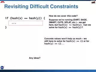
1. Revisiting Difficult Constraints How do we cover this code? Suppose we’re running (DART, SAGE,SMART, CUTE, SPLAT, etc.) – we gethere, but hash(x) != hash(y). Can wesolve for hash(x) == hash(y)? if (hash(x) == hash(y)) { ... } Concrete values won’t help us much – westill have to solve for hash(x) == C1 or forhash(y) == C2. . . Any ideas?

2. Today • A brief “digression” on causality and philosophy (of science) • Fault localization & error explanation • Renieris & Reiss: Nearest Neighbors • Jones & Harrold: Tarantula • How to evaluate a fault localization • PDGs (+ BFS or ranking) • Solving for a nearest run (not really testing)

3. Causality • When a test case fails we start debugging • We assume that the fault (what we’re really after) causes the failure • Remember RIP (Reachability, Infection, Propagation)? • What do we mean when we say that • “A causes B”?

4. Causality • We don’t know • Though it is central to everyday life – and to the aims of science • A real understanding of causality eludes us to this day • Still no non-controversial way to answer the question “does A cause B”?

5. Causality • Philosophy of causality is a fairly active area, back to Aristotle, and (more modern approaches) Hume • General agreement that a cause is something that “makes a difference” – if the cause had not been, then the effect wouldn’t have been • One theory that is rather popular with computer scientists is David Lewis’ counterfactual approach • Probably because it (and probabilistic or statistical approaches) are amenable to mathematical treatment and automation

6. Causality (According to Lewis) • For Lewis (roughly – I’m conflating his counterfactual dependency and causal dependency) • A causes B (in world w) iff • In all possible worlds that are maximally similar to w, and in which A does not take place, B also does not take place

7. Causality (According to Lewis) • Causality does not depend on • B being impossible without A • Seems reasonable: we don’t, when asking “Was Larry slipping on the banana peel causally dependent on Curly dropping it?” consider worlds in which new circumstances (Moe dropping a banana peel) are introduced

8. Causality (According to Lewis) • Many objections to Lewis in the literature • e.g. cause precedes the event in time seems to not be required by his approach • One is not a problem for our purposes • Distance metrics (how similar is world w to world w’) are problematic for “worlds” • Counterfactuals are tricky • Not a problem for program executions • May be details to handle, but no one has in-principle objections to asking how similar two program executions are • Or philosophical problems with multiple executions (no run is “privileged by actuality”)

9. Causality (According to Lewis) A d’ d A B B d’ d Yes! d < d’ B No. d > d’ Did A cause B in this program execution?

10. Formally • A predicate e is causally dependent on a predicate c in an execution a iff: • c(a)  e(a) • b . (c(b)  e(b)  (b’ . (c(b’)  e(b’))  (d(a, b) < d(a, b’))))

11. What does this have to do with automated debugging?? • A fault is an incorrect part of a program • In a failing test case, some fault is reached and executes • Causing the state of the program to be corrupted (error) • This incorrect state is propagated through the program (propagation is a series of “A causes B”s) • Finally, bad state is observable as a failure– caused by the fault

12. Fault Localization • Fault localization, then, is: • An effort to automatically find (one of the) causes of an observable failure • It is inherently difficult because there are many causes of the failure that are not the fault • We don’t mind seeing the chain of cause and effect reaching back to the fault • But the fact that we reached the fault at all is also a cause!

13. Enough! • Ok, let’s get back to testing and some methods for localizing faults from test cases • But – keep in mind that when we localize a fault, we’re really trying to automate finding causal relationships • The fault is a cause of the failure

14. Lewis and Fault Localization • Causality: • Generally agreed that explanation is about causality.[Ball,Naik,Rajamani],[Zeller],[Groce,Visser],[Sosa,Tooley],[Lewis],etc. • Similarity: • Also often assumed that successful executions that are similar to a failing run can help explain an error. [Zeller],[Renieris,Reiss][Groce,Visser],etc. • This work was not based on Lewis’ approach – it seems that this point about similarity is just an intuitive understanding most people (or at least computer scientists) share

15. Distance and Similarity • We already saw this idea at play in one version of Zeller’s delta-debugging • Trying to find the one change needed to take a successful run and make it fail • Most similar thread schedule that doesn’t cause a failure, etc. • Renieris and Reiss based a general fault localization technique on this idea – measuring distances between executions • To localize a fault, compare the failing trace with its nearest neighbor according to some distance metric

16. Renieris and Reiss’ Localization • Basic idea (over-simplified) • We have lots of test cases • Some fail • A much larger number pass • Pick a failure • Find most similar successful test case • Report differences as our fault localization “nearest neighbor”

17. Renieris and Reiss’ Localization • Collect spectra of executions, rather than the full executions • For example, just count the number of times each source statement executed • Previous work on using spectra for localization basically amounted to set difference/union – for example, find features unique to (or lacking in) the failing run(s) • Problem: many failing runs have no such features – many successful test cases have R (and maybe I) but not P! • Otherwise, localization wouldbe very easy

18. Renieris and Reiss’ Localization • Some obvious and not so obvious points to think about • Technique makes intuitive sense • But what if there are no successful runs that are very similar? • Random testing might produce runs that all differ in various accidental ways • Is this approach over-dependent on test suite quality?

19. Renieris and Reiss’ Localization • Some obvious and not so obvious points to think about • What if we minimize the failing run using delta-debugging? • Now lots of differences with original successful runs just due to length! • We could produce a very similar run by using delta-debugging to get a 1-change run that succeeds (there will actually be many of these) • Can still use Renieris and Reiss’ approach – because delta-debugging works over the inputs, not the program behavior, spectra for these runs will be more or less similar to the failing test case

20. Renieris and Reiss’ Localization • Many details (see the paper): • Choice of spectra • Choice of distance metric • How to handle equal spectra for failing/passing tests? • Basic idea is nonetheless straightforward

21. The Tarantula Approach • Jones, Harrold (and Stasko): Tarantula • Not based on distance metrics or a Lewis-like assumption • A “statistical” approach to fault localization • Originally conceived of as a visualization approach: produces a picture of all source in program, colored according to how “suspicious” it is • Green: not likely to be faulty • Yellow: hrm, a little suspicious • Red: very suspicious, likely fault

22. The Tarantula Approach

23. The Tarantula Approach • How do we score a statement in this approach? (where do all those colors come from?) • Again, assume we have a large set of tests, some passing, some failing • “Coverage entity” e (e.g., statement) • failed(e) = # tests covering e that fail • passed(e) = # tests covering e that pass • totalfailed, totalpassed = what you’d expect

24. The Tarantula Approach • How do we score a statement in this approach? (where do all those colors come from?)

25. The Tarantula Approach • Not very suspicious: appears in almost every passing test and almost every failing test • Highly suspicious: appears much more frequently in failing than passing tests

26. The Tarantula Approach mid() int x, y, z, m;1 read (x, y, z);2 m = z;3 if (y < z)4 if (x < y)5 m = y;6 else if (x < z)7 m = y;8 else9 if (x > y)10 m = y;11 else if (x > z)12 m = x;13 print (m); Simple program to computethe middle of three inputs,with a fault.

27. The Tarantula Approach Run some tests. . . Look at whether they pass or fail Look at coverage of entities mid() int x, y, z, m;1 read (x, y, z); 2 m = z;3 if (y < z)4 if (x < y)5 m = y;6 else if (x < z)7 m = y;8 else9 if (x > y)10 m = y;11 else if (x > z)12 m = x;13 print (m); 0.50.50.50.630.00.710.830.00.00.00.00.00.5 (3,3,5) (1,2,3) (3,2,1) (5,5,5) (5,3,4) (2,1,3) Compute suspiciousness using the formula Fault is indeed most suspicious!

28. The Tarantula Approach • Obvious benefits: • No problem if the fault is reached in some successful test cases • Doesn’t depend on having any successful tests that are similar to the failing test(s) • Provides a ranking of every statement, instead of just a set of nodes – directions on where to look next • Numerical, even – how much more suspicious is X than Y? • The pretty visualization may be quite helpful in seeing relationships between suspicious statements • Is it less sensitive to accidental features of random tests, and to test suite quality in general? • What about minimized failing tests here?

29. Tarantula vs. Nearest Neighbor • Which approach is better? • Once upon a time: • Fault localization papers gave a few anecdotes of their technique working well, showed it working better than another approach on some example, and called it a day • We’d like something more quantitative (how much better is this technique than that one?) and much less subjective!

30. Evaluating Fault Localization Approaches Which of theseis the “best”fault localization? • Fault localization tools produce reports • We can reduce a report to a set (or ranking) of program locations • Let’s say we have three localization tools which produce • A big report that includes the fault • A much smaller report, but the actual fault is not part of it • Another small report, also not containing the fault

31. Evaluating a Fault Localization Report • Idea (credit to Renieris and Reiss): • Imagine an “ideal” debugger, the perfect programmer • Starts reading the report • Expands outwards from nodes (program locations) in the report to associated nodes, adding those at each step • If a variable use is in the report, looks at the places it might be assigned • If code is in the report, looks at the condition of any ifs guarding that code • In general, follows program (causal) dependencies • As soon as a fault is reached, recognizes it!

32. Evaluating a Fault Localization Report • Score the reports according to • How much code the ideal debugger would read, starting from the report • Empty report: score = 0 • Every line in the program: score = 0 • Big report, containing the bug? mediocre score • Small report, far from the bug? bad score • Small report, “near” the bug? good score • Report is the fault: great score (0.9) 0.4 0.8 0.2 0.9

33. Evaluating a Fault Localization Report • Breadth-first search of Program Dependency Graph (PDG) starting from fault localization: • Terminate the search when a real fault is found • Score is proportion of the PDG that is not explored during the breadth-first search • Score near 1.00 = report includes only faults

34. Details of Evaluation Method PDG 12 total nodes in PDG

35. Details of Evaluation Method PDG 12 total nodes in PDG Report Fault

36. Details of Evaluation Method PDG 12 total nodes in PDG Report + 1 Layer BFS Fault

37. Details of Evaluation Method PDG 12 total nodes in PDG Report + 1 Layer BFS STOP: Real fault discovered Fault

38. Details of Evaluation Method PDG 12 total nodes in PDG 8 of 12 nodes not covered by BFS: score = 8/12 ~= 0.67. Report + 1 Layer BFS STOP: Real fault discovered Fault

39. Details of Evaluation Method PDG Report 12 total nodes in PDG Fault

40. Details of Evaluation Method PDG Report + 2 layers BFS 12 total nodes in PDG Fault

41. Details of Evaluation Method PDG Report + 3 layers BFS 12 total nodes in PDG Fault

42. Details of Evaluation Method PDG Report + 4 layers BFS STOP: Real fault discovered 12 total nodes in PDG Fault

43. Details of Evaluation Method PDG Report + 4 layers BFS 12 total nodes in PDG 0 of 12 nodes not covered by BFS: score = 0/12 ~= 0.00. Fault

44. Details of Evaluation Method PDG 12 total nodes in PDG 11 of 12 nodes not covered by BFS: score = 11/12 ~= 0.92. Fault = Report

45. Evaluating a Fault Localization Report • Caveats: • Isn’t a misleading report (a small number of nodes, far from the bug) actually muchworse than an empty report? • “I don’t know” vs. • “Oh, yeah man, you left your keys in the living room somewhere” (when in fact your keys are in a field in Nebraska) • Nobody really searches a PDG like that! • Not backed up by user studies to show high scores correlate to users finding the fault quickly from the report

46. Evaluating a Fault Localization Report • Still, the Renieris/Reiss scoring has been widely adopted by the testing community and some model checking folks • Best thing we’ve got, for now

47. Evaluating Fault Localization Approaches • So, how do the techniques stack up? • Tarantula seems to be the best of the test suite based techniques • Next best is the Cause Transitions approach of Cleve and Zeller (see their paper), but it sometimes uses programmer knowledge • Two different Nearest-Neighbor approaches are next best • Set-intersection and set-union are worst • For details, see the Tarantula paper

48. Evaluating Fault Localization Approaches • Tarantula got scores at the 0.99 or > level 3 times more often than the next best • Trend continued at every ranking – Tarantula was always the best approach • Also appeared to be efficient: • Much faster than Cause-Transitions approach of Cleve and Zeller • Probably about the same as the Nearest Neighbor and set-union/intersection methods

49. Evaluating Fault Localization Approaches • Caveats: • Evaluation is over the Siemens suite (again!) • But Tarantula has done well on larger programs • Tarantula and Nearest Neighbor might both benefit from larger test suites produced by random testing • Siemens is not that many tests, done by hand

50. Another Way to Do It • Question: • How good would the Nearest Neighbors method be if our test suite contained all possible executions (the universe of tests)? • We suspect it would do much better, right? • But of course, that’s ridiculous – we can’t check for distance to every possible successful test case! • Unless our program can be model checked • Leads us into next week’s topic, in a roundabout way: testing via model checking