Download
1 / 38
380 likes | 833 Views
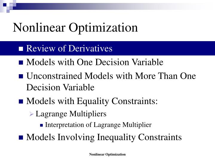
Nonlinear Optimization. Review of Derivatives Models with One Decision Variable Unconstrained Models with More Than One Decision Variable Models with Equality Constraints: Lagrange Multipliers Interpretation of Lagrange Multiplier Models Involving Inequality Constraints.

E N D
Nonlinear Optimization • Review of Derivatives • Models with One Decision Variable • Unconstrained Models with More Than One Decision Variable • Models with Equality Constraints: • Lagrange Multipliers • Interpretation of Lagrange Multiplier • Models Involving Inequality Constraints Nonlinear Optimization
Review of 1st Derivatives • Notation: • y = f(x), dy/dx = f’(x) • f(x) = c f’(x) = 0 • f(x) = xn f’(x) = n*x(n-1) • f(x) = xf’(x) = 1*x0 = 1 • f(x) = x5 f’(x) = 5*x4 • f(x) = 1/x3 f(x) = x-3 f’(x) = -3*x4 • f(x) = c*g(x)f’(x) = c*g’(x) • f(x) = 10*x2 f’(x) = 20*x • f(x) = u(x)+v(x)f’(x) = u’(x)+v’(x) • f(x) = x2 - 5xf’(x) = 2x - 5 Nonlinear Optimization
Review of 2nd Derivatives • Notation: • y = f(x), d(f’(x))/dx = d2y/dx2 = f’’(x) • f(x) = -x2 f’(x) = -2x f’’(x) = -2 • f(x) = x-3 f’(x) = -3x-4f’’(x) = 12x-5 Nonlinear Optimization
Nonlinear Optimization • Review of Derivatives • Models with One Decision Variable • Unconstrained Models with More Than One Decision Variable • Models with Equality Constraints: • Lagrange Multipliers • Interpretation of Lagrange Multiplier • Models Involving Inequality Constraints Nonlinear Optimization
Models with One Decision Variable • Requires 1st & 2nd derivative tests Nonlinear Optimization
1st & 2nd Derivative Tests • Rule 1 (Necessary Condition): • df/dx = 0 • Rule 2 (Sufficient Condition): • d2f/dx2 > 0 Minimum • d2f/dx2 < 0 Maximum Nonlinear Optimization
Maximum Example • Rule 1: • f(x) = y = -50 + 100x – 5x2 • dy/dx = 100 – 10x = 0, x = 10 • Rule 2: • d2y/dx2 = -10 • Therefore, since d2y/dx2 < 0: f(x) has a Maximum at x=10 Nonlinear Optimization
Maximum Example – Graph Solution Nonlinear Optimization
Minimum Example • Rule 1: • f(x) = y = x2 – 6x + 9 • dy/dx = 2x - 6 = 0, x = 3 • Rule 2: • d2y/dx2 = 2 • Therefore, since d2y/dx2 > 0: f(x) has a Minimum at x=3. Nonlinear Optimization
Minimum Example – Graph Solution 3 Nonlinear Optimization
Max & Min Example • Rule 1: • f(x) = y = x3/3 – x2 • dy/dx = f’(x) = x2 – 2x = 0; x = 0, 2 • Rule 2: • d2y/dx2 = f’’(x) = 2x – 2 = 0 • 2(0) – 2 = -2, f’’(x=0) = -2 • Therefore, d2y/dx2 < 0: Maximum of f(x) at x=0 • 2(2) – 2 = 2, f’’(x=2) = 2 • Therefore, d2y/dx2 > 0: Minimum of f(x) at x=2 Nonlinear Optimization
Max & Min Example – Graph Solution 2 0 Nonlinear Optimization
Example: Cubic Cost Function Resulting in Quadratic 1st Derivative • Rule 1: • f(x) = C = 10x3 – 200x2 – 30x + 15,000 • dC/dx = f’(x)= 30x2 – 400x – 30 = 0 • Quadratic Form: ax2 + bx + c Nonlinear Optimization
Rule 2: • d2y/dx2 = f’’(x) = 60x – 400 • 60(13.4) – 400 = 404 > 0 • Therefore, d2y/dx2 > 0: Minimum of f(x) at x = 13.4 • 60(-.07) – 400 = -404.2 < 0 • Therefore, d2y/dx2 < 0: Maximum of f(x) at x = -.07 Nonlinear Optimization
Cubic Cost Function – Graph Solution -.07 13.4 Nonlinear Optimization
Economic Order Quantity – EOQ • Assumptions: • Demand for a particular item is known and constant • Reorder time (time from when the order is placed until the shipment arrives) is also known • The order is filled all at once, i.e. when the shipment arrives, it arrives all at once and in the quantity requested • Annual cost of carrying the item in inventory is proportional to the value of the items in inventory • Ordering cost is fixed and constant, regardless of the size of the order Nonlinear Optimization
Economic Order Quantity – EOQ • Variable Definitions: • Let • Q represent the optimal order quantity, or the EOQ • Ch represent the annual carrying (or holding) cost per unit of inventory • Co represent the fixed ordering costs per order • D represent the number of units demanded annually Nonlinear Optimization
Economic Order Quantity – EOQ • Note: If all the previous assumptions are satisfied, then the number of units in inventory would follow the pattern in the graph below: EOQ Model Q Time Nonlinear Optimization
Economic Order Quantity – EOQ • At time = 0 after the initial delivery, the inventory level would be Q. The inventory level would then decline, following the straight line since demand is constant. When the inventory just reaches zero, the next delivery would occur (since delivery time is known and constant) and the inventory would instantaneously return to Q. This pattern would repeat throughout the year. Nonlinear Optimization
Economic Order Quantity – EOQ • Under these assumptions: • Average Inventory Level = Q/2 • Annual Carrying (or Holding) Cost = (Q/2)*Ch • The annual ordering cost would be the number of orders times the ordering cost: (D/Q)* Co • Total Annual Cost = TC = (Q/2)*Ch+(D/Q)* Co Nonlinear Optimization
Economic Order Quantity – EOQ • To find the Optimal Order Quantity, Q take the first derivative of TC with respect to Q: • (dTC/dQ) = (Ch/2) – DCoQ-2 = 0 • Solving this for Q, we find: • Q* = (2DCo/Ch)^(1/2) • Which is the Optimal Order Quaintly • Checking the second-order conditions (Rule 2 in our text), we have: • (d2TC/dQ2)= (2DCo/Q3) • Which is always > 0, since all the quantities in the expression are positive. Therefore, Q* gives a minimum value for total cost (TC) Nonlinear Optimization
Restricted Interval Problems • Step 1: • Find all the points that satisfy rules 1 & 2. These are candidates for yielding the optimal solution to the problem. • Step 2: • If the optimal solution is restricted to a specified interval, evaluate the function at the end points of the interval. • Step 3: • Compare the values of the function at all the points found in steps 1 and 2. The largest of these is the global maximum solution; the smallest is the global minimum solution. Nonlinear Optimization
Nonlinear Optimization • Review of Derivatives • Models with One Decision Variable • Unconstrained Models with More Than One Decision Variable • Models with Equality Constraints: • Lagrange Multipliers • Interpretation of Lagrange Multiplier • Models Involving Inequality Constraints Nonlinear Optimization
Unconstrained Models with More Than One Decision Variable • Requires partial derivatives Nonlinear Optimization
Example Partial Derivatives • If z = 3x2y3 • ∂z/∂x = 6xy3 • ∂z/∂y = 9y2x2 • If z = 5x3 – 3x2y2 + 7y5 • ∂z/∂x = 15x2 – 6xy2 • ∂z/∂y = -6x2y+ 35y4 Nonlinear Optimization
2nd Partial Derivatives • 2nd Partials • (∂/∂x) (∂z/∂x) = ∂2z/∂x2 • (∂/dy) (∂z/∂y) = ∂2z/∂y2 • Mixed Partials • (∂/∂x) (∂z/∂y) = ∂2z/(∂x∂y) • (∂/∂y) (∂z/∂x) = ∂2z/(∂y∂x) Nonlinear Optimization
Example 2nd Partial Derivatives • If z = 7x3 + 9xy2 + 2y5 • ∂z/∂x = 21x2 + 9y2 • ∂z/∂y = 18xy + 10y4 • ∂2z/(∂y∂x) = 18y • ∂2z/(∂x∂y) = 18y • ∂2z/∂x2 = 42x • ∂2z/∂y2 = 40y3 Nonlinear Optimization
Partial Derivative Tests • Rule 3 (Necessary Condition): • ∂f/∂x1 = 0, ∂f/∂x2 = 0, Solve Simultaneously • Rule 4 (Sufficient Condition): • If ∂2f/∂x12 > 0 • And (∂2f/∂x12)*(∂2f/∂x22) – (∂2f/(∂x1∂x2))2 > 0 • Then Minimum • If ∂2f/∂x12 < 0 • And (∂2f/∂x12)*(∂2f/∂x22) – (∂2f/(∂x1∂x2))2 > 0 • Then Maximum Nonlinear Optimization
Partial Derivative Tests • Rule 4, continued: • If (∂2f/∂x12)*(∂2f/∂x22) – (∂2f/(∂x1∂x2))2 < 0 • Then Saddle Point • If (∂2f/∂x12)*(∂2f/∂x22) – (∂2f/(∂x1∂x2))2 = 0 • Then no conclusion Nonlinear Optimization
Partial Derivative Tests • Rule 5 (Necessary Condition): • All n partial derivatives of an unconstrained function of n variables, f(x1, x2, …, xn), must equal zero at any local maximum or any local minimum point. Nonlinear Optimization
Nonlinear Optimization • Review of Derivatives • Models with One Decision Variable • Unconstrained Models with More Than One Decision Variable • Models with Equality Constraints: • Lagrange Multipliers • Interpretation of Lagrange Multiplier • Models Involving Inequality Constraints Nonlinear Optimization
Lagrange Multipliers • Nonlinear Optimization with an equality constraint • Max or Min f(x1, x2) • ST: g(x1, x2) = b • Form the Lagrangian Function: • L = f(x1, x2) + λ[g(x1, x2) – b] Nonlinear Optimization
Lagrange Multipliers • Rule 6 (Necessary Condition): • Optimization of an equality constrained function, 1st order conditions: • ∂L/∂x1= 0 • ∂L/∂x2= 0 • ∂L/∂λ= 0 Nonlinear Optimization
Lagrange Multipliers • Rule 7 (Sufficient Condition): • If rule 6 is satisfied at a point (x*1, x*2, λ*) apply conditions (a) and (b) of rule 4 to the Lagrangian function with λ fixed at a value of λ* to determine if the point (x*1, x*2) is a local maximum or a local minimum. Nonlinear Optimization
Lagrange Multipliers • Rule 8 (Necessary Condition): • For the function of n variables, f(x1, x2, …, xn), subject to m constraints to have a local maximum or a local minimum at a point, the partial derivatives of the Langrangian function with respect to x1, x2, …, xn and λ1, λ2, …, λm must all equal zero at that point. Nonlinear Optimization
Interpretation of Lagrange Multipliers • The value of the Lagrange multiplier associated with the general model above is the negative of the rate of change of the objective function with respect to a change in b. More formally, it is negative of the partial derivative of f(x1, x2) with respect to b; that is, • λ = - ∂f/∂b or • ∂f/∂b = - λ Nonlinear Optimization
Nonlinear Optimization • Review of Derivatives • Models with One Decision Variable • Unconstrained Models with More Than One Decision Variable • Models with Equality Constraints: • Lagrange Multipliers • Interpretation of Lagrange Multiplier • Models Involving Inequality Constraints Nonlinear Optimization
Models Involving Inequality Constraints • Step 1: • Assume the constraint is not binding, and apply the procedures of “Unconstrained Models with More Than One Decision Variable” to find the global maximum of the function, if it exists. (Functions that go to infinity do not have a global maximum). If this global maximum satisfies the constraint, stop. This is the global maximum for the inequality-constrained problem. If not, the constraint may be binding at the optimum. Record the value of any local maximum that satisfies the inequality constraint, and go on to Step 2. • Step 2: • Assume the constraint is binding, and apply the procedures of “Models with Equality Constraints” to find all the local maxima of the resulting equality-constrained problem. Compare these values with any feasible local maxima found in Step 1. The largest of these is the global maximum. Nonlinear Optimization