Download

1 / 35
380 likes | 570 Views
Chapter 3. Dynamic Response. Effects of Zeros and Additional Poles. Given a transfer function with 2 complex poles and 1 zero:. ζ = 0.5. The zero is located at:. The poles are located at:.

E N D
Chapter 3 Dynamic Response Effects of Zeros and Additional Poles • Given a transfer function with 2 complex poles and 1 zero: ζ=0.5 • The zero is located at: • The poles are located at: • If a is large, the zero will be far from the poles and the zero will have little effect on the response. • If a≈ 1, the value of the zero will be close to that of the real part of the poles and can be expected to have a substantial influence on the response.
Chapter 3 Dynamic Response Effects of Zeros and Additional Poles • Step response of a second-order system with zero in the LHP Overall response Original response(having no zero) Response introduced by the zero • The major effect of the zero in the LHP is to increase the overshoot. • It has very little influence on the settling time.
Chapter 3 Dynamic Response Effects of Zeros and Additional Poles • Step response of a second-order system with zero in the RHP Original response(having no zero) Overall response Response introduced by the zero • The major effect of the zero in the RHP is to depress the overshoot. • It may cause an initial undershoot (the step response starts out in the wrong direction).
Chapter 3 Dynamic Response Effects of Zeros and Additional Poles • Given a transfer function with two complex poles and one real pole: • The real pole is located at :
Chapter 3 Dynamic Response Effects of Zeros and Additional Poles • Step response of several third-order systems with ζ=0.5 ζ=0.5 • The major effect of an extra pole is to increase the rise time. • If α is large (hence far from the other poles), the extra pole have little effect on the response.
Chapter 3 Dynamic Response Summary of Effects of Pole and Zero • The poleand zero locations determine the character of the transient response. • A zero in the LHP will increase the overshoot if the zero is within a factor of 4 of the real part of the complex poles (s). • A zero in the RHP will depress the overshoot (and may cause the step response to start out in the wrong direction). • An additional pole in the LHP will increase the rise time significantly (slow down the response) if the extra pole is within a factor of 4 of the real part of the complex poles. • If the extra pole is more than a factor of 6 of the real part of the complex poles, the effect is negligible. • An additional pole in the RHP will …?
Chapter 3 Dynamic Response Stability • Consider the linear time-invariant system (LTI system). For those systems, the following condition for stability applies: “ A linear time-invariant system is said to be stable if all the roots of the transfer function denominator polynomial have negative real parts (i.e., they are all in the left half of s-plane) and is unstable otherwise. ” s< 0 s= 0 s> 0 • A system is stable if its impulse responses decay to zero and is unstable if they diverge.
Chapter 3 Dynamic Response Stability of Linear Time-Invariant Systems • Consider the linear time-invariant system whose transfer function denominator polynomial leads to the characteristic equation • Assume that the roots {pi} of the characteristic equation are real or complex, but are distinct; so that the transfer function can be given as:
Chapter 3 Dynamic Response Stability of Linear Time-Invariant Systems • The solution of the system response, found using partial fraction expansion, may be written as: • The system is stable if and only if (necessary and sufficient condition) every term in the equation above goes to zero as t ¥. for all pi • This situation will happen if all the poles of the system are strictly in the LHP.
Chapter 3 Dynamic Response Stability of Linear Time-Invariant Systems • If any LHP poles are repeated, the response will change because a polynomial in t must be included in place of Ki. However, the conclusion is the same: as t ¥, y(t) 0. for any n≥ 1 • Thus, the stability of a system can be determined by computing the location of the roots of the characteristic equation and determining whether they are all in the LHP. This is called internal stability. • If a system has any poles in the RHP, it is unstable. • If a system has non-repeated jω-axis poles, then it is said to be neutrally stable. • If the system has repeated poles on the jω axis, then it is unstable, as it results in te±jωt.
Chapter 3 Dynamic Response Routh’s Stability Criterion • The roots of the characteristic equation determine whether the system is stable or unstable. • Consider the characteristic equation • Routh’s stability criterion allows us to make certain statements about the stability of the system without actually solving for the roots of the polynomial. • Routh’s stability criterion is also useful for determining the ranges of coefficients of polynomials for stability, especially when the coefficients are in symbolic (non-numerical) form.
Chapter 3 Dynamic Response Routh’s Stability Criterion • A necessary condition for stability of the system is that all of the roots of its characteristic equation have negative real parts, which in turn requires that all the coefficients{ai} be positive. “ A necessary (but not sufficient) condition for stability is that all the coefficients of the characteristic polynomial be positive. ” “ If a system is stable, then all the coefficients of the characteristic polynomial are positive. ” • Implication pq: • If p, then q. • p implies q. • p only if q. • p is the sufficient condition for q. • q is the necessary condition for p.
Chapter 3 Dynamic Response Routh’s Stability Criterion • Once the elementary necessary conditions have been satisfied, a more powerful test is needed. • Routh in 1874 proposed a test that requires the computation of a triangular array that is a function of the coefficients of the characteristic equation. “ A system is stable if and only if all the elements in the first column of the Routh array are positive. ” “ If a system is stable then all the elements in the first column of the Routh array are positive, and vice versa. ” • Bi-Implication pq: • p ifandonly if q. • p is the sufficient and necessary conditions for q. • if p then q, and if q then p.
Chapter 3 Dynamic Response Routh’s Stability Criterion • Consider the characteristic equation • First, arrange the coefficients of the characteristic polynomial in two rows, beginning with the first and second coefficients and followed by the even-numbered and odd-numbered coefficients:
Chapter 3 Dynamic Response Routh’s Stability Criterion • Then add subsequent rows to complete the Routh array: • If the elements of the first column are all positive, then all the roots are in the LHP. • If the elements are not all positive, then the number of roots in the RHP equals the number of sign changes in the column. First column of Routh’s array
Chapter 3 Dynamic Response Example 1: Routh’s Test All the coefficients of the characteristic equation are positive the system maybe stable or maybe not. Now, we determine whether all of the roots are in the LHP
Chapter 3 Dynamic Response Example 1: Routh’s Test 2.5 0 4
Chapter 3 Dynamic Response Example 1: Routh’s Test 2 –2.4 4 3
Chapter 3 Dynamic Response Example 1: Routh’s Test • The elements of the first column are not all positive The characteristic equation has at least one RHP root • The system is unstable • There are two sign changes (+ to – and – to +) There are two poles in the RHP
Chapter 3 Dynamic Response Example 1: Routh’s Test • Roots of polynomials can also be found by using MATLAB: • Roots in the RHP, i.e.,roots with positive real parts • There are two roots of characteristic equation in the RHP • There are two unstable poles
Chapter 3 Dynamic Response Example 2: Routh’s Test Given the characteristic equation: Is the system described by this characteristic equation stable? “ If a system is stable, then all the coefficients of the characteristic polynomial are positive. ” “ If notall the coefficients of the characteristic polynomial are positive, then a system is not stable. ” p q ~q ~p
Chapter 3 Dynamic Response Example 2: Routh’s Test • There is a negative coefficient • The system is not stable • Necessary condition for stability is not even fulfilled No need to continue to Routh’s Test • Roots in the RHP, i.e.,roots with positive real parts
Chapter 3 Dynamic Response Stability Versus Parameter Range Consider the system shown below. The stability properties of the system are a function of the proportional feedback gain K. Determine the range of K over which the system is stable. • The characteristic equation • Which is the denominator of the transfer function
Chapter 3 Dynamic Response Stability Versus Parameter Range The system is stable if and only if b1 and c1 are positive.
Chapter 3 Dynamic Response Stability Versus Parameter Range Generating the step responses of the transfer function in MATLAB, for 3 different values of K:
Chapter 3 Dynamic Response Stability Versus Two Parameter Ranges Find the range of the controller gains (K, KI) so that the PI (proportional-integral) feedback system in the figure below is stable. The characteristic equation
Chapter 3 Dynamic Response K KI Stability Versus Two Parameter Ranges allowable region For the stability,
Chapter 3 Dynamic Response Special Cases for Routh’s Stability Criterion • If a first-column term in any row is zero, but the remaining terms are not zero or there is no remaining term, then the zero term is replaced by a very small positive number ε and the rest of the array is evaluated as before. Example:
Chapter 3 Dynamic Response Special Cases for Routh’s Stability Criterion • If the sign of the coefficient above the zero (ε) is the same as that below it, it indicates that there are a pair of imaginary roots. Example: + + + + The same signs above and below zero (ε) A pair of imaginary roots
Chapter 3 Dynamic Response Special Cases for Routh’s Stability Criterion • If the sign of the coefficient above the zero (ε) is opposite that below it, it indicates that there is one sign change. Example: + 1st + The opposite signs above and below ε There is one sign change The 1st root in the RHP + - Another sign change between s2 and s1 The 2nd root in the RHP 2nd + +
Chapter 3 Dynamic Response Special Cases for Routh’s Stability Criterion • If all the coefficients in any derived row are zero, it indicates that there are roots of equal magnitude lying radially opposite in the s-plane, that is, two real roots with equal magnitudes and opposite signs and/or two conjugate imaginary roots. • In such a case, the evaluation of the rest of the array can be continued by forming an auxiliary polynomial from the last nonzero row, and then using the coefficients of the derivative of this auxiliary polynomial to replace the zero row.
Chapter 3 Dynamic Response Special Cases for Routh’s Stability Criterion Example: Auxiliary polynomial from the last nonzero row Zero row Derivative of the auxiliary polynomial New Zero row is replaced • Onezero row • Radially opposite roots • No sign change • No root in the RHP
Chapter 3 Dynamic Response Special Cases for Routh’s Stability Criterion Unstable Example: Auxiliary polynomial from the last nonzero row Zero row New Derivative of the auxiliary polynomial Zero row is replaced • Onezero row • Radially opposite roots • One sign change • One root in the RHP
Chapter 3 Dynamic Response Homework 3 • No.1 • A system is given with a transfer function: Determine whether the system is stable or not. Use Routh’s stability criterion and verify with MATLAB. • No.2 • A system has a characteristic equation: Find the range of K for a stable system. • Deadline: 25.09.2012, at 07:30. • Quiz 1: 25.09.2012, around 09:15-10:30. • Lecture 1-3.