Reduction of Control Hazards (Branch) Stalls with Dynamic Branch Prediction

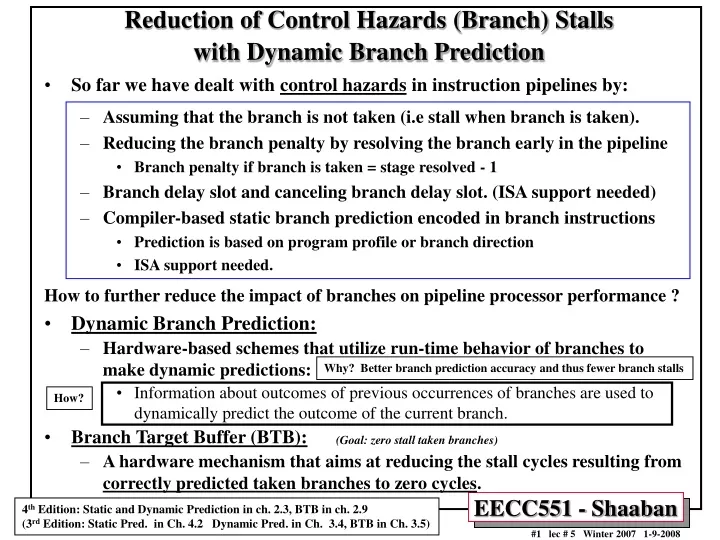
1. Reduction of Control Hazards (Branch) Stalls with Dynamic Branch Prediction • So far we have dealt with control hazards in instruction pipelines by: • Assuming that the branch is not taken (i.e stall when branch is taken). • Reducing the branch penalty by resolving the branch early in the pipeline • Branch penalty if branch is taken = stage resolved - 1 • Branch delay slot and canceling branch delay slot. (ISA support needed) • Compiler-based static branch prediction encoded in branch instructions • Prediction is based on program profile or branch direction • ISA support needed. How to further reduce the impact of branches on pipeline processor performance ? • Dynamic Branch Prediction: • Hardware-based schemes that utilize run-time behavior of branches to make dynamic predictions: • Information about outcomes of previous occurrences of branches are used to dynamically predict the outcome of the current branch. • Branch Target Buffer (BTB): • A hardware mechanism that aims at reducing the stall cycles resulting from correctly predicted taken branches to zero cycles. Why? Better branch prediction accuracy and thus fewer branch stalls How? (Goal: zero stall taken branches) 4th Edition: Static and Dynamic Prediction in ch. 2.3, BTB in ch. 2.9 (3rd Edition: Static Pred. in Ch. 4.2 Dynamic Pred. in Ch. 3.4, BTB in Ch. 3.5)

2. X = Static Prediction bit X= 0 Not Taken X = 1 Taken X Branch Encoding Static Conditional Branch Prediction • Branch prediction schemes can be classified into static (at compilation time) and dynamic (at runtime) schemes. • Static methods are carried out by the compiler. They are static because the prediction is already known before the program is executed. • Static Branch prediction is encoded in branch instructions using one prediction (or branch direction hint) bit = 0 = Not Taken, = 1 = Taken • Must be supported by ISA, Ex: HP PA-RISC, PowerPC, UltraSPARC • Two basic methods to statically predict branches at compile time: • Use the direction of a branch to base the prediction on. Predict backward branches (branches which decrease the PC) to be taken (e.g. loops) and forward branches (branches which increase the PC) not to be taken. • Profiling can also be used to predict the outcome of a branch. • A number runs of the program are used to collect program behavior information (i.e. if a given branch is likely to be taken or not) • This information is included in the opcode of the branch (one bit branch direction hint) as the static prediction. 1 2 Static prediction was previously discussed in lecture 2 4th edition: in Chapter 2.3, 3rd Edition: In Chapter 4.2

3. Static Profile-Based Compiler Branch Misprediction Rates for SPEC92 More Loops (FP has more loops) Integer Floating Point Average 15% Average 9% (i.e 91% Prediction Accuracy) (i.e 85% Prediction Accuracy) (repeated here from lecture2)

4. Dynamic Conditional Branch Prediction • Dynamic branch prediction schemes are different from static mechanisms because they utilize hardware-based mechanisms that use the run-time behavior of branches to make more accurate predictions than possible using static prediction. • Usually information about outcomes of previous occurrences of branches (branching history) is used to dynamically predict the outcome of the current branch. The two main types of dynamic branch prediction are: • One-level or Bimodal: Usually implemented as a Pattern History Table (PHT), a table of usually two-bit saturating counters which is indexed by a portion of the branch address (low bits of address). (First proposed mid 1980s) • Also called non-correlating dynamic branch predictors. • Two-Level Adaptive Branch Prediction. (First proposed early 1990s). • Also called correlating dynamic branch predictors. • To reduce the stall cycles resulting from correctly predicted taken branches to zero cycles, a Branch Target Buffer (BTB) that includes the addresses of conditional branches that were taken along with their targets is added to the fetch stage. How? Why? 1 2 BTB BTB discussed next 4th Edition: Dynamic Prediction in Chapter 2.3, BTB in Chapter 2.9 (3rd Dynamic Prediction in Chapter 3.4, BTB in Chapter 3.5)

5. Branch Target Buffer (BTB) • Effective branch prediction requires the target of the branch at an early pipeline stage. (resolve the branch early in the pipeline) • One can use additional adders to calculate the target, as soon as the branch instruction is decoded. This would mean that one has to wait until the ID stage before the target of the branch can be fetched, taken branches would be fetched with a one-cycle penalty (this was done in the enhanced MIPS pipeline Fig A.24). • To avoid this problem and to achieve zero stall cycles for taken branches, one can use a Branch Target Buffer (BTB). • A typical BTB is an associative memory where the addresses of taken branch instructions are stored together with their target addresses. • The BTB is is accessed in Instruction Fetch (IF) cycle and provides answers to the following questions while the current instruction is being fetched: • Is the instruction a branch? • If yes, is the branch predicted taken? • If yes, what is the branch target? • Instructions are fetched from the target stored in the BTB in case the branch is predicted-taken and found in BTB. • After the branch has been resolved the BTB is updated. If a branch is encountered for the first time a new entry is created once it is resolved as taken. BTB Goal 1 2 3 Goal of BTB: Zero stall taken branches 4th Edition: BTB in Chapter 2.9 (pages 121-122) (3rd BTB in Chapter 3.5)

6. Basic Branch Target Buffer (BTB) Fetch instruction from instruction memory (I-L1 Cache) Is the instruction a branch? (for address match) Branch Address Branch Target if predicted taken Instruction Fetch IF Branch Taken? Branch Targets BTB is accessed in Instruction Fetch (IF) cycle 0 = NT = Not Taken 1 = T = Taken i.e target Goal of BTB: Zero stall taken branches

7. BTB Lookup BTB Operation One more stall to update BTB Penalty = 1 + 1 = 2 cycles Here, branches are assumed to be resolved in ID Update BTB

8. Branch Penalty CyclesUsing A Branch-Target Buffer (BTB) Base Pipeline Taken Branch Penalty = 1 cycle (i.e. branches resolved in ID) i.e In BTB? No Not Taken Not Taken 0 Assuming one more stall cycle to update BTB Penalty = 1 + 1 = 2 cycles

9. N Low Bits of Branch Address PHT Entry: One Bit 0 = NT = Not Taken 1 = T = Taken PHT T NT T . . . 1 0 Predictor = Saturating Counter NT Basic Dynamic Branch Prediction • Simplest method: (One-Level or Non-Correlating) • A branch prediction buffer or Pattern History Table (PHT) indexed by low address bits of the branch instruction. • Each buffer location (or PHT entry or predictor) contains one bit indicating whether the branch was recently taken or not • e.g 0 = not taken , 1 =taken • Always mispredicts in first and last loop iterations. • To improve prediction accuracy, two-bit prediction is used: • A prediction must miss twice before it is changed. • Thus, a branch involved in a loop will be mispredicted only once when encountered the next time as opposed to twice when one bit is used. • Two-bit prediction is a specific case of n-bit saturating counter incremented when the branch is taken and decremented when the branch is not taken. • Two-bit saturating counters (predictors) are usually always used based on observations that the performance of two-bit PHT prediction is comparable to that of n-bit predictors. Saturating counter 2N entries or predictors (Smith Algorithm, 1985) Why 2-bit Prediction? The counter (predictor) used is updated after the branch is resolved Smith Algorithm 4th Edition: In Chapter 2.3 (3rd Edition: In Chapter 3.4)

10. 2-bit saturating counters One-Level Bimodal Branch Predictors Pattern History Table (PHT) Most common one-level implementation 2-bit saturating counters (predictors) Sometimes referred to as Decode History Table (DHT) or Branch History Table (BHT) High bit determines branch prediction 0 = NT = Not Taken 1 = T = Taken N Low Bits of Table (PHT) has 2N entries (also called predictors) . Not Taken (NT) 0 0 0 1 1 0 1 1 Example: For N =12 Table has 2N = 212 entries = 4096 = 4k entries Number of bits needed = 2 x 4k = 8k bits Taken (T) Update counter after branch is resolved: -Increment counter used if branch is taken - Decrement counter used if branch is not taken What if different branches map to the same predictor (counter)? This is called branch address aliasing and leads to interference with current branch prediction by other branches and may lower branch prediction accuracy for programs with aliasing.

11. Taken (T) 11 10 Not Taken (NT) 0 0 0 1 1 0 1 1 Taken (T) Taken (T) Taken (T) Not Taken (NT) Taken (NT) Predict Taken Predict Taken Predict Not Taken Predict Not Taken 00 01 Taken (T) 01 11 10 00 Not Taken (NT) Not Taken (NT) Not Taken (NT) Not Taken (NT) Basic Dynamic Two-Bit Branch Prediction: Two-bit Predictor State Transition Diagram (in textbook) Or Two-bit saturating counter predictor state transition diagram (Smith Algorithm): Not Taken (NT) Taken (T) The two-bit predictor used is updated after the branch is resolved

12. Prediction Accuracy of A 4096-Entry Basic One-Level Dynamic Two-Bit Branch Predictor N=12 2N = 4096 FP Misprediction Rate: Integer average 11% FP average 4% (Lower misprediction rate due to more loops) Integer Has, more branches involved in IF-Then-Else constructs the FP

13. MIPS From The Analysis of Static Branch Prediction : MIPS Performance Using Canceling Delay Branches 70% Static Branch Prediction Accuracy (repeated here from lecture2)

14. Prediction Accuracy of Basic One-Level Two-Bit Branch Predictors: N=12 2N = 4096 N= All branch address bits FP 4096-entry buffer (PHT) Vs. An Infinite Buffer Under SPEC89 Integer Conclusion: SPEC89 programs do not have many branches that suffer from branch address aliasing (interference) when using a 4096-entry PHT. Thus increasing PHT size (which usually lowers aliasing) did not result in major prediction accuracy improvement.

15. Correlating Branches Recent branches are possibly correlated: The behavior of recently executed branches affects prediction of current branch. Example: Branch B3 is correlated with branches B1, B2. If B1, B2 are both not taken, then B3 will be taken. Using only the behavior of one branch cannot detect this behavior. Occur in branches used to implement if-then-else constructs Which are more common in integer than floating point code Here aa = R1 bb = R2 DSUBUI R3, R1, #2 ; R3 = R1 - 2 BNEZ R3, L1 ; B1 (aa!=2) DADD R1, R0, R0 ; aa==0 L1: DSUBUI R3, R2, #2 ; R3 = R2 - 2 BNEZ R3, L2 ; B2 (bb!=2) DADD R2, R0, R0 ; bb==0 L2: DSUBUI R3, R1, R2 ; R3=aa-bb BEQZ R3, L3 ; B3 (aa==bb) B1 if (aa==2) aa=0; B2 if (bb==2) bb=0; B3 if (aa!==bb){ B1 not taken (not taken) B2 not taken (not taken) (not taken) B3 taken if aa=bb aa=bb=2 B3 in this case

16. Correlating Two-Level Dynamic GAp Branch Predictors • Improve branch prediction by looking not only at the history of the branch in question but also at that of other branches using two levels of branch history. • Uses two levels of branch history: • First level (global): • Record the global pattern or history of the m most recently executed branches as taken or not taken. Usually an m-bit shift register. • Second level (per branch address): • 2m prediction tables, each table entry has n bit saturating counter. • The branch history pattern from first level is used to select the proper branch prediction table in the second level. • The low N bits of the branch address are used to select the correct prediction entry (predictor)within a the selected table, thus each of the 2m tables has 2N entries and each entry is 2 bits counter. • Total number of bits needed for second level = 2m x n x 2N bits • In general, the notation: GAp (m,n) predictor means: • Record last m branches to select between 2m history tables. • Each second level table uses n-bit counters (each table entry has n bits). • Basic two-bit single-level Bimodal BHT is then a (0,2) predictor. Last Branch 0 =Not taken 1 = Taken m-bit shift register Branch History Register (BHR) 1 BHR 2 Pattern History Tables (PHTs) 4th Edition: In Chapter 2.3 (3rd Edition: In Chapter 3.4)

17. Organization of A Correlating Two-level GAp (2,2) Branch Predictor (N= 4) Low 4 bits of address (n = 2) n= 2 m= 2 Global (1st level) Second Level Adaptive Pattern History Tables (PHTs) GAp High bit determines branch prediction 0 = Not Taken 1 = Taken per address (2nd level) Selects correct Entry (predictor) in table m = # of branches tracked in first level = 2 Thus 2m = 22 = 4 tables in second level N = # of low bits of branch address used = 4 Thus each table in 2nd level has 2N = 24 = 16 entries n = # number of bits of 2nd level table entry = 2 Number of bits for 2nd level = 2m x n x 2N = 4 x 2 x 16 = 128 bits 00 01 10 11 Selects correct table First Level Branch History Register (BHR) (2 bit shift register) Branch History Register (BHR) (m = 2) GAp (m,n) here m= 2 n =2 Thus Gap (2, 2)

18. if (d==0) d=1; if (d==1) BNEZ R1, L1 ; branch b1 (d!=0) DADDIU R1, R0, #1 ; d==0, so d=1 L1: DADDIU R3, R1, # -1 BNEZ R3, L2 ; branch b2 (d!=1) . . . L2: Dynamic Branch Prediction: Example One Level One Level with one-bit table entries (predictors) : NT = 0 = Not Taken T = 1 = Taken

19. if (d==0) d=1; if (d==1) Dynamic Branch Prediction: Example (continued) BNEZ R1, L1 ; branch b1 (d!=0) DADDIU R1, R0, #1 ; d==0, so d=1 L1: DADDIU R3, R1, # -1 BNEZ R3, L2 ; branch b2 (d!=1) . . . L2: Two level GAp(1,1) m= 1 n= 1

20. Prediction Accuracy of Two-Bit Dynamic Predictors Under SPEC89 N = 10 N = 12 Basic Basic Correlating Two-level Single (one) Level Gap (2, 2) FP n= 2 m= 2 Integer

21. A Two-Level Dynamic Branch Predictor Variation: MCFarling's gshare Predictor gshare = global history with index sharing • McFarling noted (1993) that using global history information might be less efficient than simply using the address of the branch instruction, especially for small predictors. • He suggests using both global history (BHR) and branch address by hashing them together. He proposed using the XOR of global branch history register (BHR) and branch address since he expects that this value has more information than either one of its components. The result is that this mechanism outperforms GAp scheme by a small margin. • This mechanism uses less hardware than GAp, since both branch history (first level) and pattern history (second level) are kept globally. • The hardware cost for k history bits is k + 2 x 2k bits, neglecting costs for logic. gshare is one one the most widely implemented two level dynamic branch prediction schemes

22. gshare Predictor Branch and pattern history are kept globally. History and branch address are XORed and the result is used to index the pattern history table. (BHR) Here: m = N = k First Level: XOR (bitwise XOR) Index the second level 2-bit saturating counters (predictors) Second Level: (PHT) One Pattern History Table (PHT) with 2k entries (predictors) gshare = global history with index sharing

23. gshare Performance gshare GAp One Level (Gap) (One Level)

24. Hybrid Predictors(Also known as tournament or combined predictors) • Hybrid predictors are simply combinations of two (most common) or more branch prediction mechanisms. • This approach takes into account that different mechanisms may perform best for different branch scenarios. • McFarling presented (1993) a number of different combinations of two branch prediction mechanisms. • He proposed to use an additional 2-bit counter selector array which serves to select the appropriate predictor for each branch. • One predictor is chosen for the higher two counts, the second one for the lower two counts. The selector array counter used is updated as follows: • If the first predictor is wrong and the second one is right the selector counter used counter is decremented, • If the first one is right and the second one is wrong, the selector counter used is incremented. • No changes are carried out to selector counter used if both predictors are correct or wrong. Predictor Selector Array Counter Update

25. A Generic Hybrid Predictor BHR Branch Prediction Which branch predictor to choose Usually only two predictors are used (i.e. n =2) e.g. As in Alpha, IBM POWER 4, 5, 6

26. 11 10 01 00 Use P1 Use P2 X X MCFarling’s Hybrid Predictor Structure The hybrid predictor contains an additional counter array (selector array) with 2-bit up/down saturating counters. Which serves to select the best predictor to use. Each counter in the selector array keeps track of which predictor is more accurate for the branches that share that counter. Specifically, using the notation P1c and P2c to denote whether predictors P1 and P2 are correct respectively, the selector counter is incremented or decremented by P1c-P2c as shown. Both wrong P2 correct P1 correct Both correct Selector Counter Update Selector Array e.g gshare e.g One level Branch Address Here two predictors are combined (N Low Bits) (Current example implementations: IBM POWER4, 5, 6)

27. MCFarling’s Hybrid Predictor Performance by Benchmark (Single Level) (Combined)

28. Processor Branch Prediction Examples Processor ReleasedAccuracyPrediction Mechanism Cyrix 6x86 early '96 ca. 85% PHT associated with BTB Cyrix 6x86MX May '97 ca. 90% PHT associated with BTB AMD K5 mid '94 80% PHT associated with I-cache AMD K6 early '97 95% 2-level adaptive associated with BTIC and ALU Intel Pentium late '93 78% PHT associated with BTB Intel P6 mid '96 90% 2 level adaptive with BTB PowerPC750 mid '97 90% PHT associated with BTIC MC68060 mid '94 90% PHT associated with BTIC DEC Alpha early '97 95% Hybrid 2-level adaptive associated with I-cache HP PA8000 early '96 80% PHT associated with BTB SUN UltraSparc mid '95 88%int PHT associated with I-cache 94%FP S+D S+D S+D PHT = One Level S+D : Uses both static (ISA supported) and dynamic branch prediction