Download
1 / 25
250 likes | 410 Views
Latent Concepts and the Number Orthogonal Factors in Latent Semantic Analysis. Georges Dupret georges.dupret@laposte.net. Abstract. We seek insight into Latent Semantic Indexing by establishing a method to identify the optimal number of factors in the reduced matrix for representing a keyword.

E N D
Latent Concepts and the Number Orthogonal Factors in Latent Semantic Analysis Georges Dupret georges.dupret@laposte.net
Abstract • We seek insight into Latent Semantic Indexing by establishing a method to identify the optimal number of factors in the reduced matrix for representing a keyword. • By examining the precision, we find that lower ranked dimensions identify related terms and higher-ranked dimensions discriminate between the synonyms.
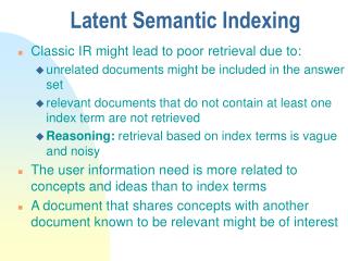
Introduction • The task of retrieving the documents relevant to a user query in a large text database is complicated by the fact that different authors use different words to express the same ideas or concepts. • Methods related to Latent Semantic Analysis interpret the variability associated with the expression of a concept as a noise, and use linear algebra techniques to isolate the perennial concept from the variable noise.
Introduction • In LSA, the SVD (singular value decomposition) technique is used to decompose a term by document matrix to a set of orthogonal factors. • A large number of factor weights provide an approximation close to the original term by document matrix but retains too much noise. • On the other hand, if too many factors are discarded, the information loss is too large. • The objective is to identify the optimal number of orthogonal factors.
Bag-of-words representation • Each documents is replaced by a vector of its attributes which are usually the keywords present in the document. • This representation can be used to retrieve document relevant to a user query: A vector representation is derived from the query in the same way as regular documents and then compared with the database using a suitable measure of distance or similarity.
Latent Semantic Analysis • LSI is one of the few methods which successfully overcome the vocabulary noise problem because it takes into account synonymy and polysemy. • Not accounting for synonymy leads to under-estimate the similarity between related documents, and not accounting for polysemy leads to erroneously finding similarities. • The idea behind LSI is to reduce the dimension of the IR problem by projecting the D documents by N attributes matrix A to an adequate subspace of lower dimension.
Latent Semantic Analysis • SVD of the D × N matrix A: A = UΔVT (1) U,V: orthogonal matrices Δ: a diagonal matrix with elements σ1,…,σp, where p=min(D, N) and σ1 ≧σ2 ≧… ≧σp-1 ≧σp • The closest matrix A(k) of dimension k < rank(A) is obtained by setting σi =0 for i > k. A(k) = U(k) × Δ(k) × V(k)T (2)
Latent Semantic Analysis • Then we compare documents in a k dimensional subspace based on A(k). The projection of the original document representation gives AT ×U(k) × Δ(k)-1 = V(k) (3) the same operation on the query vector Q Q(k) = QT ×U(k) × Δ(k)-1 (4) • The closest document to query Q is identified by a dissimilarity function dk(., .): (5)
Covariance Method • Advantage: be able to handle databases of several hundred of thousands of documents. • If D is the number of documents, Ad the vector representing the dth document and Ā the mean of these vectors, the covariance matrix is written: (6) this matrix being symmetric, the singular value decomposition can be written: C= VΔVT (7)
Covariance Method • Reducing Δ to the k more significant singular values, we can project the keyword space into a k dimensional subspace: (A|Q) → (A|Q)V(k)Δ= (A(k)|Q(k)) (8)
Embedded Concepts • Sending the covariance matrix onto a subspace of fewer dimension implies a loss of information. • It can be interpreted as the merging of keywords meaning into a more general concept. ex: “cat” and “mouse” → “mammal” → ”animal” • How many singular values are necessary for a keyword to be correctly distinguished from all others in the dictionary? • What’s the definition of “correctly distinguished”?
Correlation Method • The correlation matrix S of A is defined based on the covariance matrix C: (9) • Using the correlation rather than the covariance matrix results in a different weighting of correlated keywords, the justification of the model remaining otherwise identical.
Keyword Validity • The property of SVD: (10) • The rank k approximation S(k) of S can be written (11) with k ≦ N. S(N) = S.
Keyword Validity • We can argue the following argument: the k-order approximation of the correlation matrix correctly represents a given keyword only if this keyword is more correlated to itself than to any other attribute. • For a given keyword α this condition is written (12) • A keyword is said to be “valid” of rank k if k-1 is the largest value for which Eq.(12) is not verified, then k is the validity rank of the keyword.
Experiments • Data: REUTERS (21,578 articles) and TREC5 (131,896 articles generated 1,822,531 “documents”) databases. • Pre-processing: • using the Porter algorithm to stem words • removing the keywords appearing in either more or less than two user specified thresholds. • mapping documents to vectors by TFIDF.
First Experiment • The claim: a given keyword is correctly represented by a rank k approximation of the correlation matrix if k is at least equal to the validity rank of the keyword. • Experiment method: • Select a keyword, for example africa, and extract all the documents containing it. • Produce a new copy of these documents, in which we replace the selected keyword by an new one. ex: replace africa by afrique (French)
First Experiment • Add these new documents to the original database, and the keyword afrique to the vocabulary. • Compute the correlation matrix and SVD of this extended, new database. Note that afrique and africa are perfect synonyms. • Send the original database to the new subspace and issue a query for afrique. We hope to find documents containing africa first.
First Experiment Figure 1: Keyword africa is replaced by afrique: Curves corresponding to ranks 450 and 500 start with a null precision and remain under the curves of lower validity ranks.
First Experiment Table 1: Keywords Characteristics
First Experiment Note: the drop in precision is low after we reach the validity rank, but still present. As usual, the validity rank is precisely defined: the drop in precision is observed as soon as the rank reaches 400.
First Experiment Figure 3: keyword network is replaced by reseau: Precision is 100% until the validity rank and deteriorates drastically beyond it.
First Experiment • This experiment shows the relation between the “concept” associated with afrique (or any other concept) and the actual keyword. • For low rank approximations S(k), augmenting the number of orthogonal factors helps identifying the “concept” common to both afrique and africa, while orthogonal factors beyond the validity rank help distinguish between the keyword and its synonym.
Second Experiment Figure 4: Ratios R and hit = N/G for keyword afrique. Validity rank is 428.
Third Experiment Figure 5: vocabulary of 1201 keywords in REUTERS db. Figure 6: vocabulary of 2486 keywords in TREC db.
Conclusion • We examined the dependence of the Latent Semantic structure on the number of orthogonal factors in the context of the Correlation Method. • We analyzed the claim that LSA provides a method to take account of synonymy. • We propose a method to determine the number of orthogonal factors for which a given keyword best represents an associated concept. • Further directions might include the extension to multiple keywords queries.