Download
1 / 53
530 likes | 641 Views
Machine Learning CS 165B Spring 2012. Course outline. Introduction (Ch. 1) Concept learning (Ch. 2) Decision trees (Ch. 3) Ensemble learning Neural Networks (Ch. 4) …. Schedule. Homework 1 due today Homework 2 on decision trees will be handed out Thursday 4/19; due Wednesday 5/2

E N D
Course outline • Introduction (Ch. 1) • Concept learning (Ch. 2) • Decision trees (Ch. 3) • Ensemble learning • Neural Networks (Ch. 4) • …
Schedule • Homework 1 due today • Homework 2 on decision trees will be handed out Thursday 4/19; due Wednesday 5/2 • Project choices by Friday 4/20 • Topic of discussion section
Projects • Projects proposals are due by Friday 4/20. • 2-person teams • If you want to define your own project: • Submit a 1-page proposal with references and ideas • Needs to have a significant Machine Learning component • You may do experimental work, theoretical work, a combination of both or a critical survey of results in some specialized topic. • Originality is not mandatory but is encouraged. • Try to make it interesting!
Decision tree learning • Decision tree representation • Most popular method for representing discrete TE’s • Decision tree represents disjunction of conjunctions • of attribute values • More general H-representation than in concept learning • ID3 learning procedure based on • Entropy of set of +/- TEs • Information gain from splitting set with use of attribute • Greedy, hill-climbing algorithm • Characterization of ID3 algorithm and its search space • Overfitting issue • Generalizations of basic procedure
Outlook sunny overcast rain Humidity Wind Yes high normal strong weak No Yes No Yes Decision Trees • Decision tree to represent learned target functions • Each internal node tests an attribute • Each branch corresponds to attribute value • Each leaf node assigns a classification • Can be representedby logical formulas
Representation in decision trees • Example of representing rule in DT’s: • if outlook = sunny AND humidity = normal • OR • if outlook = overcast • OR • if outlook = rain AND wind = weak • then playtennis
Applications of Decision Trees • Instances describable by a fixed set of attributes and their values • Target function is discrete valued • 2-valued • N-valued • But can approximate continuous functions • Disjunctive hypothesis space • Possibly noisy training data • Errors, missing values, … • Examples: • Equipment or medical diagnosis • Credit risk analysis • Calendar scheduling preferences
Top-Down Construction • Main loop: • 1. Choose the “best” decision attribute (A) for next node • 2. Assign A as decision attribute for node • 3. For each value of A, create new descendant of node • 4. Sort training examples to leaf nodes • 5. If training examples perfectly classified, STOP, Else iterate over new leaf nodes • Grow tree just deep enough for perfect classification • If possible (or can approximate at chosen depth) • Which attribute is best?
A1 A2 A1 A2 29+, 35- 29+, 35- f t t f 11+, 2- 21+, 5- 18+, 33- 8+, 30- Choosing Best Attribute? • Consider 64 examples, 29+ and 35- • Which one is better? • Which is better? 29+, 35- 29+, 35- f t t f 25+, 5- 14+, 16- 4+, 30- 15+, 19-
Entropy • A measure for • uncertainty • purity • information content • Information theory: optimal length code assigns (- log2p) bits to message having probability p • S is a sample of training examples • p+ is the proportion of positive examples in S • p- is the proportion of negative examples in S • Entropy of S: average optimal number of bits to encode information about certainty/uncertainty about S Entropy(S) = p+(-log2p+) + p-(-log2p-)= -p+log2p+- p-log2p- • Can be generalized to more than two values
Entropy • Entropy can also be viewed as measuring • purity of S, • uncertainty in S, • information in S, … • E.g.: values of entropy for p+=1, p+=0, p+=.5 • Easy generalization to more than binary values • Sum over pi *(-log2 pi) , i=1,n • i is + or – for binary • i varies from 1 to n in the general case
A1 A2 A1 A2 29+, 35- 29+, 35- f t t f 11+, 2- 21+, 5- 18+, 33- 8+, 30- Choosing Best Attribute? • Consider 64 examples (29+,35-) and compute entropies: • Which one is better? • Which is better? E(S)=0.993 E(S)=0.993 29+, 35- 29+, 35- f t t f 0.650 0.997 0.522 0.989 25+, 5- 14+, 16- 4+, 30- 15+, 19- E(S)=0.993 E(S)=0.993 0.619 0.708 0.937 0.742
E(S)=0.993 E(S)=0.993 29+, 35- 29+, 35- f t t f 0.650 0.997 A1 A1 A2 A2 0.522 0.989 25+, 5- 14+, 16- 4+, 30- 15+, 19- E(S)=0.993 E(S)=0.993 29+, 35- 29+, 35- f t t f 0.708 0.619 0.742 0.937 21+, 5- 11+, 2- 8+, 30- 18+, 33- Information Gain • Gain(S,A): reduction in entropy after choosing attr. A Gain: 0.000 Gain: 0.395 Gain: 0.265 Gain: 0.121
Gain function • Gain is measure of how much can • Reduce uncertainty • Value lies between 0,1 • What is significance of • gain of 0? • example where have 50/50 split of +/- both before and after discriminating on attributes values • gain of 1? • Example of going from “perfect uncertainty” to perfect certainty after splitting example with predictive attribute • Find “patterns” in TE’s relating to attribute values • Move to locally minimal representation of TE’s
9+, 5- E=0.940 9+, 5- E=0.940 Wind Strong Weak 3+, 3-E=1.000 6+, 2-E=0.811 Determine the Root Attribute 9+, 5- E=0.940 9+, 5- E=0.940 Humidity Low High 6+, 1-E=0.592 3+, 4-E=0.985 Gain (S, Wind) = 0.048 Gain (S, Humidity) = 0.151 Gain (S, Temp) = 0.029 Gain (S, Outlook) = 0.246
Sort the Training Examples 9+, 5- {D1,…,D14} Ssunny= {D1,D2,D8,D9,D11} Gain (Ssunny, Humidity) = .970 Gain (Ssunny, Temp) = .570 Gain (Ssunny, Wind) = .019 Outlook Sunny Overcast Rain {D1,D2,D8,D9,D11} 2+, 3- {D3,D7,D12,D13} 4+, 0- {D4,D5,D6,D10,D15} 3+, 2- Yes ? ?
Final Decision Tree for Example Outlook Sunny Rain Overcast Humidity Yes Wind High Weak Normal Strong No Yes No Yes
Hypothesis Space Search by ID3 • Hypothesis space (all possible trees) is complete! • Target function is included in there
Hypothesis Space Search in Decision Trees • Conduct a search of the space of decision trees which • can represent all possible discrete functions. • Goal: to find the best decision tree • Finding a minimal decision tree consistent with a set of data • is NP-hard. • Perform a greedy heuristic search: hill climbing without • backtracking • Statistics-based decisions using all data
Hypothesis Space Search by ID3 • Hypothesis space is complete! • H is space of all finite DT’s (all discrete functions) • Target function is included in there • Simple to complex hill-climbing search of H • Use of gain as hill-climbing function • Outputs a single hypothesis (which one?) • Cannot assess all hypotheses consistent with D (usually many) • Analogy to breadth first search • Examines all trees of given depth and chooses best… • No backtracking • Locally optimal ... • Statistics-based search choices • Use all TE’s at each step • Robust to noisy data
Restriction bias vs. Preference bias • Restriction bias (or Language bias) • Incomplete hypothesis space • Preference (or search) bias • Incomplete search strategy • Candidate Elimination has restriction bias • ID3 has preference bias • In most cases, we have both a restriction and a preference bias.
Inductive Bias in ID3 • Preference for short trees, and for those with high information gain attributes near the root • Principle of Occam's razor • prefer the shortest hypothesis that fits the data • Justification • Smaller likelihood of a short hypothesis fitting the data at random • Problems • Other ways to reduce random fits to data • Size of hypothesis based on the data representation • Minimum description length principle
Overfitting the Data • Learning a tree that classifies the training data perfectly may • not lead to the tree with the best generalization performance. • - There may be noise in the training data the tree is fitting • - The algorithm might be making decisions based on • very little data • A hypothesish is said to overfit the training data if the is • another hypothesis, h’, such thathhas smaller error than h’ • on the training data but h has larger error on the test data than h’. On training accuracy On testing Complexity of tree
Overfitting in Decision Trees • Consider adding noisy training example (should be +): • What effect on earlier tree? Outlook Sunny Overcast Rain Humidity Yes Wind Strong Weak High Normal
Outlook Rain Sunny Overcast 1,2,8,9,11 3,7,12,13 4,5,6,10,14 2+,3- 4+,0- 3+,2- Humidity Yes Wind Strong Weak High Normal Yes Wind No No Strong Weak Yes No Overfitting - Example Noise or other coincidental regularities
Avoiding Overfitting • Two basic approaches • - Prepruning: Stop growing the tree at some point during • construction when it is determined that there is not enough • data to make reliable choices. • - Postpruning: Grow the full tree and then remove nodes • that seem not to have sufficient evidence. (more popular) • Methods for evaluating subtrees to prune: • - Cross-validation: Reserve hold-out set to evaluate utility (more popular) • - Statistical testing: Test if the observed regularity can be • dismissed as likely to be occur by chance • - Minimum Description Length: Is the additional complexity of • the hypothesis smaller than remembering the exceptions ? • This is related to the notion of regularization that we will see • in other contexts– keep the hypothesis simple.
Reduced-Error Pruning • A post-pruning, cross validation approach • - Partition training data into “grow” set and “validation” set. • - Build a complete tree for the “grow” data • - Until accuracy on validation set decreases, do: • For each non-leaf node in the tree • Temporarily prune the tree below; replace it by majority vote. • Test the accuracy of the hypothesis on the validation set • Permanently prune the node with the greatest increase • in accuracy on the validation test. • Problem: Uses less data to construct the tree • Sometimes done at the rules level General Strategy: Overfit and Simplify
Rule post-pruning • Allow tree to grow until best fit (allow overfitting) • Convert tree to equivalent set of rules • One rule per leaf node • Prune each rule independently of others • Remove various preconditions to improve performance • Sort final rules into desired sequence for use
Example of rule post pruning • IF (Outlook = Sunny) ^ (Humidity = High) • THEN PlayTennis = No • IF (Outlook = Sunny) ^ (Humidity = Normal) • THEN PlayTennis = Yes Outlook Sunny Overcast Rain Humidity Wind Yes Strong Weak High Normal
Extensions of basic algorithm • Continuous valued attributes • Attributes with many values • TE’s with missing data • Attributes with associated costs • Other impurity measures • Regression tree
Continuous Valued Attributes • Create a discrete attribute from continuous variables • E.g., define critical Temperature = 82.5 • Candidate thresholds • chosen by gain function • can have more than one threshold • typically where values change quickly (80+90)/2 (48+60)/2
Attributes with Many Values • Problem: • If attribute has many values, Gain will select it (why?) • E.g. of birthdates attribute • 365 possible values • Likely to discriminate well on small sample • For sample of fixed size n, and attribute with N values, as N -> infinity • ni/N -> 0 • - pi*log pi -> 0 for all i and entropy -> 0 • Hence gain approaches max value
Attributes with many values • Problem: Gain will select attribute with many values • One approach: use GainRatio instead Entropy of the partitioning Penalizes higher number of partitions where Si is the subset of S for which A has value vi (example of Si/S = 1/N: SplitInformation = log N)
Unknown Attribute Values • What if some examples are missing values of attribute A? • Use training example anyway, sort through tree • if node n tests A, assign most common value of A among other examples sorted to node n • assign most common value of A among other examples with same target value • assign probability pi to each possible value vi of A • assign fraction pi of example to each descendant in tree • Classify test instances with missing values in same fashion • Used in C4.5
Attributes with Costs • Consider • medical diagnosis: BloodTest has cost $150, Pulse has a cost of $5. • robotics, Width-From-1ft has cost 23 sec., from 2 ft 10s. • How to learn a consistent tree with low expected cost? • Replace gain by • Tan and Schlimmer (1990) • Nunez (1988) where w [0, 1] determines importance of cost
Gini Index • Another sensible measure of impurity(i and j are classes) • After applying attribute A, the resulting Gini index is • Gini can be interpreted as expected error rate
Gini Index . . . . . . Attributes: color, border, dot Classification: triangle, square
. . . . . . Gini Index for Color . . . . . . red Color? green yellow
Decision Trees as Features • Rather than using decision trees to represent the target function, use small decision trees as features • When learning over a large number of features, learning decision trees is difficult and the resulting tree may be very large (over fitting) • Instead, learn small decision trees, with limited depth. • Treat them as “experts”; they are correct, but only on a small region in the domain. • Then, learn another function over these as features.
Regression Tree • Similar to classification • Use a set of attributes to predict the value (instead of a class label) • Instead of computing information gain, compute the sum of squared errors • Partition the attribute space into a set of rectangular subspaces, each with its own predictor • The simplest predictor is a constant value
r5 r4 r3 r2 r1 Rectilinear Division • A regression tree is a piecewise constant function of the input attributes X2 X1 t1 r5 r2 X1 t3 X2 t2 r3 t2 r4 r1 X2 t4 t3 t1 X1
| LS | å D = - a I ( LS , A ) var { y } var { y } | | y LS y LS | LS | a a Growing Regression Trees • To minimize the square error on the learning sample, the prediction at a leaf is the average output of the learning cases reaching that leaf • Impurity of a sample is defined by the variance of the output in that sample: I(LS)=vary|LS{y}=Ey|LS{(y-Ey|LS{y})2} • The best split is the one that reduces the most variance:
Regression Tree Pruning • Exactly the same algorithms apply: pre-pruning and post-pruning. • In post-pruning, the tree that minimizes the squared error on VSis selected. • In practice, pruning is more important in regression because full trees are much more complex (often all objects have a different output values and hence the full tree has as many leaves as there are objects in the learning sample)
When Are Decision Trees Useful ? • Advantages • Very fast: can handle very large datasets with many attributes • Flexible: several attribute types, classification and regression problems, missing values… • Interpretability: provide rules and attribute importance • Disadvantages • Instability of the trees (high variance) • Not always competitive with other algorithms in terms of accuracy
History of Decision Tree Research • Hunt and colleagues in Psychology used full search decision • trees methods to model human concept learning in the 60’s • Quinlan developed ID3, with the information gain heuristics • in the late 70’s to learn expert systems from examples • Breiman, Friedmans and colleagues in statistics developed • CART (classification and regression trees simultaneously • A variety of improvements in the 80’s: coping with noise, • continuous attributes, missing data, non-axis parallel etc. • Quinlan’s updated algorithm, C4.5 (1993) is commonly used (New:C5) • Boosting (or Bagging) over DTs is a good general purpose algorithm