Download
1 / 29
290 likes | 373 Views
Congestion Estimation in Floorplanning. Supervisor: Evangeline F. Y. YOUNG by Chiu Wing SHAM. Overview. Introduction Background Congestion Modeling Experimental Results Future Works. Introduction. Motivations: 80% of the clock cycle consumed by interconnects

E N D
Congestion Estimation in Floorplanning Supervisor: Evangeline F. Y. YOUNG by Chiu Wing SHAM
Overview • Introduction • Background • Congestion Modeling • Experimental Results • Future Works
Introduction • Motivations: • 80% of the clock cycle consumed by interconnects • Interconnect optimization becomes the major concern in floorplanning • Appropriate interconnect estimation is required in floorplanning
Major Role of Floorplanning • Minimization of chip area • Optimization of interconnect cost • Wirelength • Timing delay • Routability • Others: • Heat dissipation • Noise reduction • Power consumption
Congestion Planning • Congestion planning is important to circuit design • Excessive congestion may result in a local shortage of routing resources • A large expansion in area • Failure in achieving timing closure • Congestion modeling • Given a packing and netlist • Estimating the congestion and routability instead of real routing
Congestion Model A The probability that wire k passing through this grid, Pk(x,y) =4/6 =0.67
Congestion Model A Congestion of the grid (x,y) - Expected number of wires passing through the grid (x,y), weight(x,y):
Limitations • Model A assumes that all feasible routes have the same probability of being selected • In real cases, the routes with less bends should have a higher probability of being selected The probability that wire k passing through this grid, Pk(x,y) =8/24 =0.33
Congestion Model B where distk(x, y) is the distance from the source of wire k to the grid (x, y) and cntk(r) is the number of grids in the division that is r grids from the source. Congestion of the grid (x,y) due to wire k - the probability of wire k pass through the grid (x,y), Pk(x,y):
Limitations • Routing resources: • Both models assume that routing resources are equal at different locations • Routing resources should be different at different locations in real cases • Wirelength: • Both models assume that all nets are routed in their shortest Manhattan distance • Some nets may be routed with detours in real cases
Our Approaches • Congestion Model A*: • Based on model A • Routing resources can be different at different locations • Congestion Model B*: • Based on model B • Routing resources can be different at different locations • Congestion Model C: • Based on model B* • Routing resources can be different at different locations • Each net may be routed with detours
Congestion Model A* • Considering routing resources
Congestion Model A* • Notations: • res(x,y): relative routing resources at the grid (x, y) • Lk(x,y): the set of feasible routes for wire k passing through the grid (x,y) • Lk: the set of all feasible routes for wire k • Gk(l): the set of grids that the route l of wire k will pass through • wk(l): the weight of each feasible route l • Equations:
Congestion Model B* • Considering routing resources
Congestion Model B* • Notations: • res(x,y): relative routing resources at grid (x, y) • distk(x,y): the distance from the source of wire k to the grid (x,y) • divk(r): the set of grids that are r grids from the source of wire k • Equation
Congestion Model C • Considering routing resources • Each net may be routed with detours
Congestion Model C • Notations: • res(x,y): relative routing resources at the grid (x, y) • dist(x,y): the distance from the the grid (0, 0) to the grid (x,y) • divk(r): the set of grids that are r grids from the grid (0,0) of wire k • CRk: the set of divisions located in the compulsory region • ORk: the set of divisions located in the optional region • : degrade factor for the grids outside the SMB region • : degrade factor for the grids in the optional region • d(i, j, k, l): the distance between the grid (i, j) and (k, l)
Congestion Model C Equation: Compulsory Region (divk(dist(x, y)) CRk): Optional Region (divk(dist(x, y)) ORk):
Implementation • Floorplanning: • Representations: SP • Heuristics: Simulated Annealing • Cost function: Weighted sum of wirelength and number of over-congested grid • Routing • Cadence’s WROUTE
Experimental Results Test cases:
Future works • Limitations of congestion model C • Too many parameters (, ) are used • Longer running time • Limitations of representation • Packed closely together