Download
1 / 23
230 likes | 301 Views
Interdecadal Trend of Prediction Skill in an Ensemble AMIP Experiment. T. Nakaegawa, M. Kanamitsu ECPC SIO UCSD and T. M. Smith NCDC NESDIS NOAA. Backgrounds.

E N D
Interdecadal Trend of Prediction Skill in an Ensemble AMIP Experiment T. Nakaegawa, M. KanamitsuECPC SIO UCSD and T. M. Smith NCDC NESDIS NOAA
Backgrounds The operational 5-month lead forecasts had high skill over the U.S. during the very strong 1997-98 El Niño episode (Barnston et al. 1999). The skill is high during events of large interannual variability in SST, such as El Niño and La Niña episodes (Brankovic and Palmer 2000). Dynamical seasonal forecast is primarily a boundary value problem, because its skill is expected to depend on the nature of the external forcing, namely SSTs. The interannual variability of SST are known as an important factor of the skill:
Lower Activities 1920 1960 Decadal Variation in ENSO In observations, the occurrence of El Niño and the Southern Oscillation (ENSO) was reported to be significantly lower during 1920-1960 (Torrence and Compo 1998; Kestin et al. 1998), which may contribute to the decadal trend in prediction skill. Fig. The Niño 3 SST time series and local wavelet power spectrum. (Wavelet software was provided by C. Torrence and G. Compo)
Previous works: • Potential predictability of soil moisture over the U.S. may be a function of time, based on significant changes in the behavior of the time series (Stern and Miyakoda 1995). • Potential predictability of the 200hPa height was found higher in 1976-1988 than in 1955-1988 (Sugi et al. 1997). Previous Works and Objectives Objectives: This study presents the relation between forecast skill and temporal variance of SST using 50-year climate simulations forced with observed SST. 500hPa geopotential height for DJF
Contents • Introduction • Model, Data, and Analysis • Results • Difference in ACCs of DJF 500hPa height • Variance ratio of the DJF anomalous SST • Discussion • Physical processes • Interdecadal change in the variance • Summary
Experiments • Model: GSM based on NCEP SFM • Resolution: T62L28 with reduced grids • Integration period: 52 years, from 1950 to 2001 • Ensemble size: 10 • SST & Sea ice: a data set for ERA40 Experiments and Data Data • Additional SST:ERSST (Smith and Reynolds 2003) HadISST (Rayner et al. 1996) • SOI: CRU, UEA (Ropelewski and Jones 1987) • Geopotential height:NCEP-NCAR reanalysis (R-1) (Kalnay et al.1996)
Potential ACC The ACC of the simulation is computed according to Sardeshmukh et al. (2000) with "a perfect model" assumption, and is expressed as: where is the signal-to-noise ratio, n is the ensemble number, x the state vector in an ensemble member, < x > ensemble mean. Fig. PotentialACC curve
ACCs of 500hPa Height for Each Decade (1) ACCs (f; bottom-right) have typical features such as high values in the Tropics and teleconnection areas. The skill of the seasonal forecast improves from 1950s to 1990s over most of the global domain. Fig. Difference in ACC for different decades. ACC(a decade)-ACC(50yr)
Tropics Extratropics Small differences were found in the Topics. Larger negative ones were found over the subtropical zones, especially the Pacific subtropical zone and North America until 1970’s. ACCs of 500hPa Height for Each Decade (2) Fig. Potential ACC
Temporal Variance of DJF SST The variances in 1950s were small in almost all oceans. The large differences disappeared after 1980s. The variances clearly increased with time, especially in the tropical ocean and Antarctic ocean. Fig. Surface temperature variance for DJF for each decadal period. Var(a decade)/Var(1990s)
1950s Physical Processes The difference of ACCs shows patterns symmetric to the equator, especially over eastern and western Pacific. These patterns resemble those of the warm events minus cold events composite of the wind anomaly (Lau and Nath 2000). Increasing precipitation due to SSTA excites the Rossby wave. Fig. Top:Difference in ACCs, bottom:warm - cold composite of 850hPa horizontal wind of R-1
Other Interdecadal Variabilities ENSO Indices Niño-3 SST variance has upward trend since 1950 ( Xue et al. 2003) Similar trends are found in the standard deviation of SOI (Kestin et al. 1998; Torrence and Compo 1998). Other variables • central equatorial Pacific Rainfall (Kestin et al. 1998) • Indian monsoon (Torrence and Webster 1997) • the tropical Pacific sea level (Smith 2000) • the Darwin sea level pressure(Xue et al. 2003)
0.2% 6.0% Southern Oscillation Index The simulated trend of SOI well reproduced the observed SOI (0.78) . The variances of both the SOI are small in 1950s and 1960s and have an increasing trend. The increasing rate of variance in the simulation is significantly larger than that in the observation. Fig. The time variation of SOI temporal variance in the time window of 11-years for DJF.
0.2% 4.3% PNA pattern The two patterns were similar, but the amplitude in the simulation is smaller than that of the observation. The temporal correlation coefficient was 0.22. The time variations of 11-year temporal variance from the both the data sets had an increasing trend. Fig. The REOF second mode of observed 500hPa geopotential height and the first mode of the ensemble mean of the simulations.
58.6% 0.4% 500hPa Height over the continental U.S The largest number of the data there since 1950s is used in R-1. Therefore R-1 data are less affected by R-1 systematic error. No statistically significant trend in the variance of R-1 is found but the trend in the variance in the simulation clearly increased: Fig. The time variation of 500hPa height over continental U.S. temporal variance in the time window of 11-years for DJF.
Decadal Temporal Variance of Tropical SST Similar trends among the three data sets were found after 1950s, but the trends in earlier years were different, especially before 1900. Fig. Interdecadal change of the decadal temporal variance of tropical SST over 80W-180W, 10S-10N from ERA40, HadISST and ERSST since late 1800’s.
Issues remaining The change in observation system can affect the variance in the NCEP/NCAR Reanalysis. None knows how the variance changes. The large discrepancy of the variance in SST is likely due to very minimal SST observations available at a time, although it is debatable. The skill in a historical run since late 1800’s will be significantly influenced on by the discrepancy.
Summary (1) A distinct decadal positive trend in the ACC was found. This trend is shown to be consistent with the positive trend in the interdecadal timescale temporal variance of SST. The geographical pattern of the differences of ACC between each decade and the 50-year period resembles the Matsuno-Gill pattern, suggesting the increase in ACC is due to the Rossby wave excitation induced by the anomalous diabatic heating caused by the increasing anomalous SST.
Summary (2) A similar interdecadal trend in the variance of the Southern Oscillation Index and the Pacific North America pattern were found in both the observation and the simulation. The interdecadal trend in the variance of 500hPa geopotential height over the continental U.S., however, existed only in the simulation. Decadal temporal variance of tropical SST has similar trends among the three data sets after 1950s, but different trends in earlier years.
Trend of the Mean of 500hPa Height Trend can affect the variance. The contribution of the trend is approximately as Vt=83m^2 for R-1 out of 200m^2 Vt=53m^2 for R-1 out of 50 to 100 m^2 The contribution reaches about 50%.
Temporal Variance of DJF SST The temporal variance increases with time in the tropical eastern Pacific. The variance is large in the Pacific subtropical zone in 1970s. Fig. Surface temperature variance for DJF for each decadal period.Var(a decade)/Var(1990s)
Temporal Variance of DJF 500hPa Height The temporal variance increase with time in the subtropical eastern Pacific. The dipole-like pattern was found. The temporal variance was high in mid- and high latitude during the four decadal periods. Fig. 500hPa height variance of each decadal period for DJF. Var(a decade)/Var(1990s) These characteristics is not consistent with those of the simulation.