Q uantum C omputer O verview

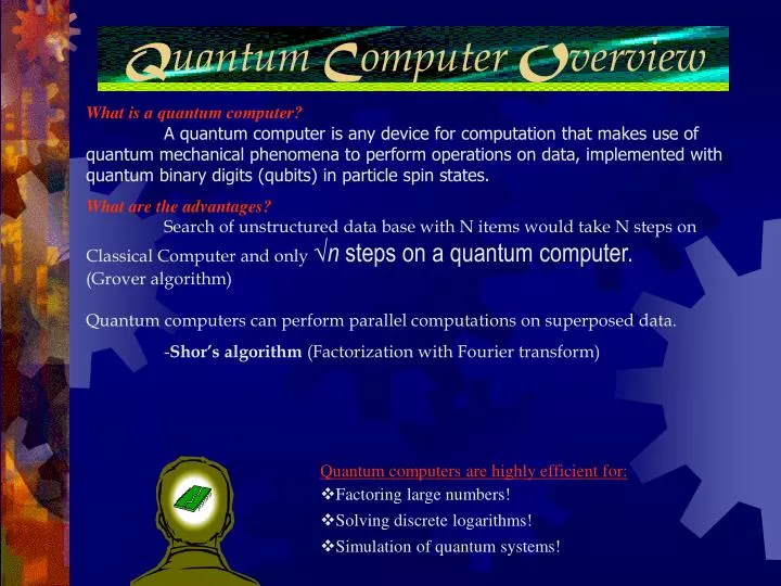
1. QuantumComputerOverview What is a quantum computer? A quantum computer is any device for computation that makes use of quantum mechanical phenomena to perform operations on data, implemented with quantum binary digits (qubits) in particle spin states. What are the advantages? Search of unstructured data base with N items would take N steps on Classical Computer and only √n steps on a quantum computer. (Grover algorithm) Quantum computers can perform parallel computations on superposed data. -Shor’s algorithm (Factorization with Fourier transform) Quantum computers are highly efficient for: • Factoring large numbers! • Solving discrete logarithms! • Simulation of quantum systems!

2. Quantum Registers, Ket Notation Eigenstates Complex Amplitudes Sign affects relative phase factor Adds up to 1! Typical state vector of single-particle system: Where |α|2 + |β|2 = 1 and |α|2 or |β|2 give the probability of observing each state. Since all possible 2n binary states of an n-qubit quantum register can be superposed, the register can be described by a state vector: |Ψ> = α0|…000> + α1|…001> + α2|…010> + α3|…011> + … + αn|?> …or in a column with 2n entries correlating binary states to amplitudes. Ψ1 = α1|0> ± β1|1> Example: (With arbitrary amplitudes – |a+bi| is √(a2+b2))

3. Quantum Array Notation vs. Classical = EXOR operation = Wire a P=a = Product operation b Q=ac b c R=c All quantum circuits are reversible (have a one-to-one correspondence between input and output vectors), so quantum array gates do not have an implicate direction like standard Boolean gates. Example (Toffoli EXOR-middle):

4. Quantum Permutative Gates Overview All quantum gates are represented by unitary matrices that define transformations on qubits. Permutative gates are gates whose unitary matrices are simply permutative matrices. Five major types and their tautological equivalents: -Inverter (NOT – also a quantum primitive) -Feynman (Controlled-NOT) -Toffoli (Controlled-Controlled-NOT) -Fredkin (Controlled-Swap) -Swap These gate-matrices can also be described by how many inputs are fed to the output with no transformations, in which case they are said to be “k-through.” A reversible gate with n inputs/outputs is described by a 2n*2n matrix.

5. Inverter (NOT) X a P 0 1 0 0 1 1 0 P=a 1 Schematic: (zero-through) Unitary Matrix: Logic:

6. Feynmann (CNOT) 00 01 10 11 00 01 10 11 00 00 01 01 (P, Q)=(a, a b) 10 10 a P 11 11 b Q 1 0 0 0 0 0 0 1 0 0 1 0 0 1 0 0 1 0 0 0 0 1 0 0 0 0 0 1 0 0 1 0 a P (P, Q)=(a b, b) b Q Schematic: (one-through) Unitary Matrices: Logic: EXOR-Down EXOR-Up

7. Toffoli (CCNOT) a P b Q c R 000 001 010 011 100 101 110 111 000 1 0 0 0 0 0 0 0 0 1 0 0 0 0 0 0 0 0 1 0 0 0 0 0 0 0 0 1 0 0 0 0 0 0 0 0 1 0 0 0 0 0 0 0 0 1 0 0 0 0 0 0 0 0 0 1 0 0 0 0 0 0 1 0 001 010 011 (P, Q)=(a, b), R=ab c 100 101 110 111 Schematic of EXOR-down: (two-through) Unitary Matrix: Logic:

8. Fredkin (CSWAP) a P b Q c R 000 001 010 011 100 101 110 111 000 1 0 0 0 0 0 0 0 0 1 0 0 0 0 0 0 0 0 1 0 0 0 0 0 0 0 0 1 0 0 0 0 0 0 0 0 1 0 0 0 0 0 0 0 0 0 1 0 0 0 0 0 0 1 0 0 0 0 0 0 0 0 0 1 001 010 011 P=a, Q=ab ac, R=ac ab 100 or 101 P=a, Q=if (a=1) then c else b, R= if (a=1) then b else c 110 111 Schematic of Fredkin-Up: (one-through) Unitary Matrix: Logic:

9. Swap Gate a P a P 00 01 10 11 00 b Q b Q a 01 P 10 b Q 11 1 0 0 0 0 0 1 0 0 1 0 0 0 0 0 1 Schematic: (zero-through) Feynmann Gate Realizations: Unitary Matrix: Logic: P=b, Q=a

10. Universal Controlled Gate a P ? U b Q P=a; if a=0 then Q=b; if a=1 then Q=U(b)

11. Matrices Overview … + 1 0 0 i 1 0 0 -i 1 0 0 -i 1 0 0 i … = In = … … … … … 1 0 0 1 = 1 0 0 0 1 0 0 0 1 * (1+0) (0+0) (0+0) (0+1) a b c d = = I2 Testing for Unitary Matrix U: (Example: Phase gate matrix) -Identity Matrix (Square matrix with “1” in entries along main diagonal, “0s” elsewhere): 1) Take the hermitian transpose U+ of U: -Permutation Matrix: Square matrix with entry of “1” in each row/column 2) Verify that U*U+ = I (the corresponding n*n identity matrix): -Inverse Matrix: Square matrix A-1 of A such that AA-1=A-1A=In -Orthogonal Matrix: Square matrix Q whose transpose is its inverse: QQT=QTQ=In Where: 1) a2+c2 = 1 2) b2+d2 = 1 3) ab+cd = 0

12. Standard Product 00 01 10 11 a P 00 01 * b Q 1 0 0 0 0 0 0 1 0 1 0 0 0 0 1 0 1 0 0 0 0 0 1 0 0 1 0 0 0 0 0 1 10 11 Feynmann-Down Swap 1 0 0 0 0 1 0 0 0 0 0 1 0 0 1 0 Unitary Matrix of Circuit (Permutative) The product A*B of two quantum gate-matrices A and B in a serial connection is used to derive their collective unitary matrix. Example: = =

13. Kronecker Product X Pauli-X gate 00 01 10 11 a P 00 b Q 01 0 0 0 -i 0 0 i 0 0 -i 0 0 i 0 0 0 Y 10 Pauli-Y gate 11 0 1 1 0 0 -i i 0 Unitary Matrix of Circuit The Kronecker product A B of two quantum gate-matrices A and B in a parallel connection is used to derive their collective unitary matrix. Example: X (NOT) Y = =

14. Matrix Vector u1 + v1 un+ vn u1 un |u> + |v> = … |u> = … (Corresponds toCn where un = an+bni) y The ket represents a vector z x A vector is a line segment with a direction and magnitude spanning some set of axes. In quantum mechanics, a complex vector space of n dimensions (axes) is denoted Cn (Hilbert space). Column Notation for Vectors: (With entries representing coordinates of the terminal point in complex vector space) Vector Addition: Dual/Adjoint Vector <u| of Ket Vector |u>: (Transpose column and conjugate entries) <u| = |u>† = [u1*, …, un*]

15. Truly Quantum Primitives X Z V Y H S Most truly quantum primitive gates cannot be decomposed into simpler matrix operators. They include complex entries to reflect state vector amplitudes rather than only standard bits, thus introducing quantum phenomena into reversible circuits (and can also transform qubit inputs into superposed states). Hadamard Pauli-X (NOT) Pauli-Y Pauli-Z Phase V (√NOT)

16. Hadamard, Phase, V (√NOT) H V S 1 1 1 1 -1 1 0 0 i √2 1 1+i 1-i 1-i 1+i 2 Unitary Matrices:

17. Pauli- X (NOT), Y, Z Z X Y 0 -i i 0 0 1 1 0 1 0 0 -1 Unitary Matrices:

18. Simple Circuit Equivalences 2 V V = X 1 1+i 1-i 1-i 1+i 0 1 1 0 1 0 0 1 = 2 2 1 2 0 0 2 1 1 1 -1 H H = = = √2 1 2 U U+ = U*U+ = I

19. Karnaugh Maps and Testing A B P 0 0 0 0 1 1 1 0 1 1 1 0 A A 00 01 10 11 00 01 10 11 B B 00 00 1 1 1 1 1 1 1 1 01 01 1 1 1 1 1 1 1 1 10 10 0 0 0 0 0 0 0 0 A 0 1 B 11 11 0 1 0 0 0 0 0 0 0 0 0 1 0 1 In testing for constant or balanced Boolean functions, 2 tries is the best-case scenario for a regular computer while n/2+1 tries is the worst (for a function with n possible output bits). A quantum computer requires only one step using the Deutsch-Jozsa algorithm. Truth Table (Displays input/output function) EXOR Operation: Balanced Functionf(n): Karnaugh Map (Displays input/output “coordinates”) EXOR Operation:

20. Bloch Sphere!! Z |0› 1 Ψ 2θ x y z = -1 -1 sin 2θ × cos φ sin 2θ × sin φ cos 2θ 0 φ X Y 1 1 |1› √NOT -1 NOT *On the Bloch sphere, a qubit’s state vector is described as |Ψ> = cosθ |0> + eiφ sinθ |1> for –π/2 ≤ θ < π/2and 0 ≤ φ < 2π *The corresponding Bloch vector’s terminal point on the sphere’s surface is given by the coordinates:

21. Ternary Logic 1 0 0 0 1 0 0 0 1 (0° rotation of axis on qubit) (120° rotation of axis on qubit) (240° rotation of axis on qubit) |0> = |1> = |2> = 1 1 1 1 aa2 1 a2a Chrestenson Gate = basic ternary NOT (where a=ei(2π/3)): CH = Ternary logic uses three basic bits: 0, 1, and 2. Ternary quantum registers can have 3n superposed states for n-qubit inputs. Thus, the state vector would be: Ψ = α|0> + β|1> + γ|2> where -Ternary NOT gates include +1, +2, (01), (02), and (12) with parentheses denoting permutations on single-bit inputs (in addition to equivalent √NOT gates)

22. Design Realizations Proposed Quantum Computer Architectures: Criteria: (DiVincenzo checklist) • Superconductor arrays • Ion traps • Nuclear magnetic resonance (NMR) on solutions of molecules • Solid-state NMR • Quantum dot surfaces • Cavity quantum electrodynamics (CQED) structures • Molecular magnets • Physically scalable (qubits can be increased) • Qubits can be initialized to some values • Operates much faster than decoherence time • Computer uses quantum gates and logic HΨ(x,t) = iħ[dΨ(x,t)/dt] • Has a means of reading qubits Phenomena: -Superposition: “Blend” of eigenstates in QM system (QM database searching) -Entanglement: Instantaneous particle correlation (QM teleportation, communication) -Interference: Disruption of QM systems (QM parallelism, joint computations) -Non-clonability: Impossible to copy unknown QM state (QM cryptography)

23. Conclusion “If you put crap into a computer, nothing comes out of it but crap. But this crap, having passed through a very expensive machine, is somehow enobled and no-one dares criticize it.” -Pierre Gallois